Samples instead of individual values
Although control charts for individual values are sometimes used, it is more common to examine samples from a process at regular intervals rather than individual values. There are a few reasons:
- It is easier and cheaper to make measure several measurements at once -- for example
to take a sample of 12 items from a production
line every 2 hours than to measure a single item every 10 minutes.
- The control limits at 3 standard deviations on each side of the mean work best
when the distribution of values is symmetric. The corresponding limits
on a control chart for sample means depend less on the distribution of the
individual measurements -- sample means always have a more symmetric distribution
than the distribution of individual values.
- There are two ways in which a process can go out of control. Special causes may either change the process mean or they may cause the spread of values to increase. From each sample, we can estimate both location and spread. This makes it easier to separately examine the process for changes in location and spread.
Control limits for means
We first consider a control chart to detect whether the mean output level is changing. This is based on a run chart of the means of successive samples.
Sample means vary less from sample to sample than individual values, so control limits may be drawn much closer to the target mean. This control chart is therefore more sensitive to changes in the process mean over time.
The properties of samples and, in particular, sample means will be examined in detail in later chapters. At this stage, we state without proof that the appropriate control limits for the means of samples of size n are...
![]()
where
![]() and
s
are estimates of the mean and standard deviation of individual values when the process is
in control. These control limits should be distinguished carefully from the corresponding
control limits for single values,
and
s
are estimates of the mean and standard deviation of individual values when the process is
in control. These control limits should be distinguished carefully from the corresponding
control limits for single values,
![]()
Since sample means are less variable, their control limits are closer to the process mean than the control limits for single values.
Training data
In order to obtain control limits, we must know the mean and standard deviation
of the measurements when the process is 'in control'. We usually estimate
![]() and
s
from 'training samples' in which great care is taken to avoid special causes.
and
s
from 'training samples' in which great care is taken to avoid special causes.
The process mean,
![]() is estimated by the mean value from the training samples.
is estimated by the mean value from the training samples.
The process standard deviation is not however estimated by the standard deviation of the values in the training samples. Instead, it is usually based on the standard deviations within each of the training samples. With k training samples, we will denote the standard deviations in the samples by s1, s2, ..., sk. The most commonly used estimate of s is...

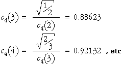
where the value c4 is a constant that depends on the sample size in each sample, n. Its value may be obtained from tables or using the formulae

The second part of this formula allows the value of c4 for sample size n to be obtained from its value for sample size n - 1, as illustrated below.

(An alternative estimate of s that is occasionally used is

Although this second estimate is better when the data have a fairly symmetric distribution, the earlier estimate is more 'robust' to problems in the training data.)
The diagram below shows thickness of paint primer in mils (an imperial measurement equal to one thousandth of an inch), measured from a sample of 10 items each morning and afternoon for 5 successive mornings and afternoons. We will regard these data as a training set from which we obtain control limits for later samples of primer thickness.
(In practice, there are usually more training samples, but we use a small real data set for illustration.)
The control limits that are initially shown are those for a run chart of individual values -- mean ± 3 standard deviations for the 50 values in the training data.
Use the scroll bar to display the samples that were measured over the next 15 half-days. No values are outside the 3-standard deviations limits, so we would conclude that the process is in control.
Now click the checkbox Show Means. The raw values in the samples are dimmed and the sample means are displayed, joined by blue lines. The sample means are considerably less variable than the raw values, so the control limits are redrawn closer to the centre line.
Based on the means, we again conclude that there is no evidence of a shift in the process mean.
As in control charts for individual values, additional triggers can be used that depend on several successive means. These are defined in the same way as those in control charts for individual values. For example, six successive sample means either increasing or decreasing suggest that there might be a special cause.