UQ MATH2504
Programming of Simulation, Analysis, and Learning Systems
(Semester 2 2022)
This is an OLDER SEMESTER.
Go to current semester
Unit 8: A Taste of Machine Learning
Up to now most of the course dealt with writing explicit instructions for a computer to perform. For example, sorting using a very specified algorithm such as bubble sort or quicksort. Yet, in recent years more and more computer programming involves using "code" that has been automatically trained and not explicitly designed and coded. This is the domain of machine learning, deep learning, and in general artificial intelligence.
Machine learning is all about training mathematical models on a computer in order to classify data, predict outcomes, estimate relationships, summarize data, control complex processes, and more. Deep learning can be viewed as a form of machine learning based on deep learning models. We will mostly focus on general machine learning. At UQ, see the course COMP4702 for a general introductory machine learning course. Further, STAT3007 is specialized deep learning course. There are multiple other courses that deal with theoretical aspects of machine learning such as STAT3006 and parts of STAT4401.
Machine learning activities are often dichotomized into two broad categories, supervised learning, and unsupervised learning. With supervised learning, data is assumed to be available as $(x, y)$ pairs where each feature vector $x$ is labeled via $y$. In the case of unsupervised learning, one only observes data points $x$ and tries to find relationships between the various elements, variables, or coordinates of $x$.
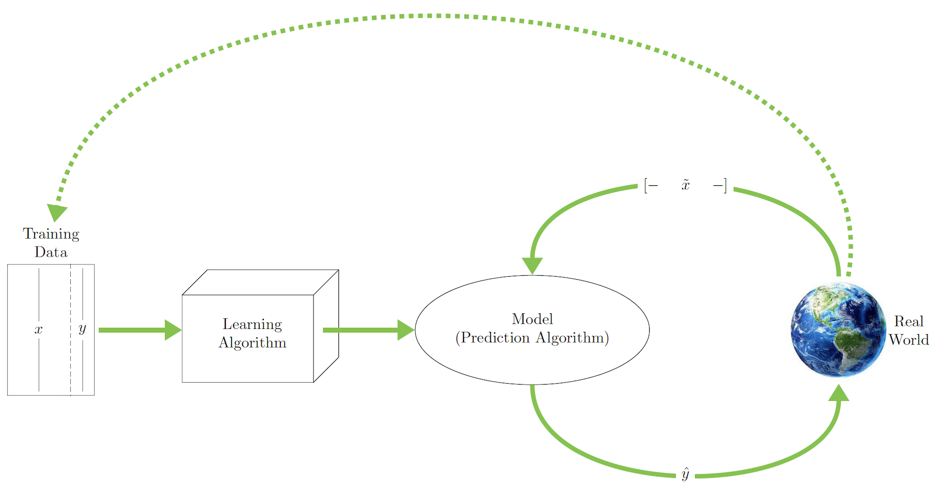
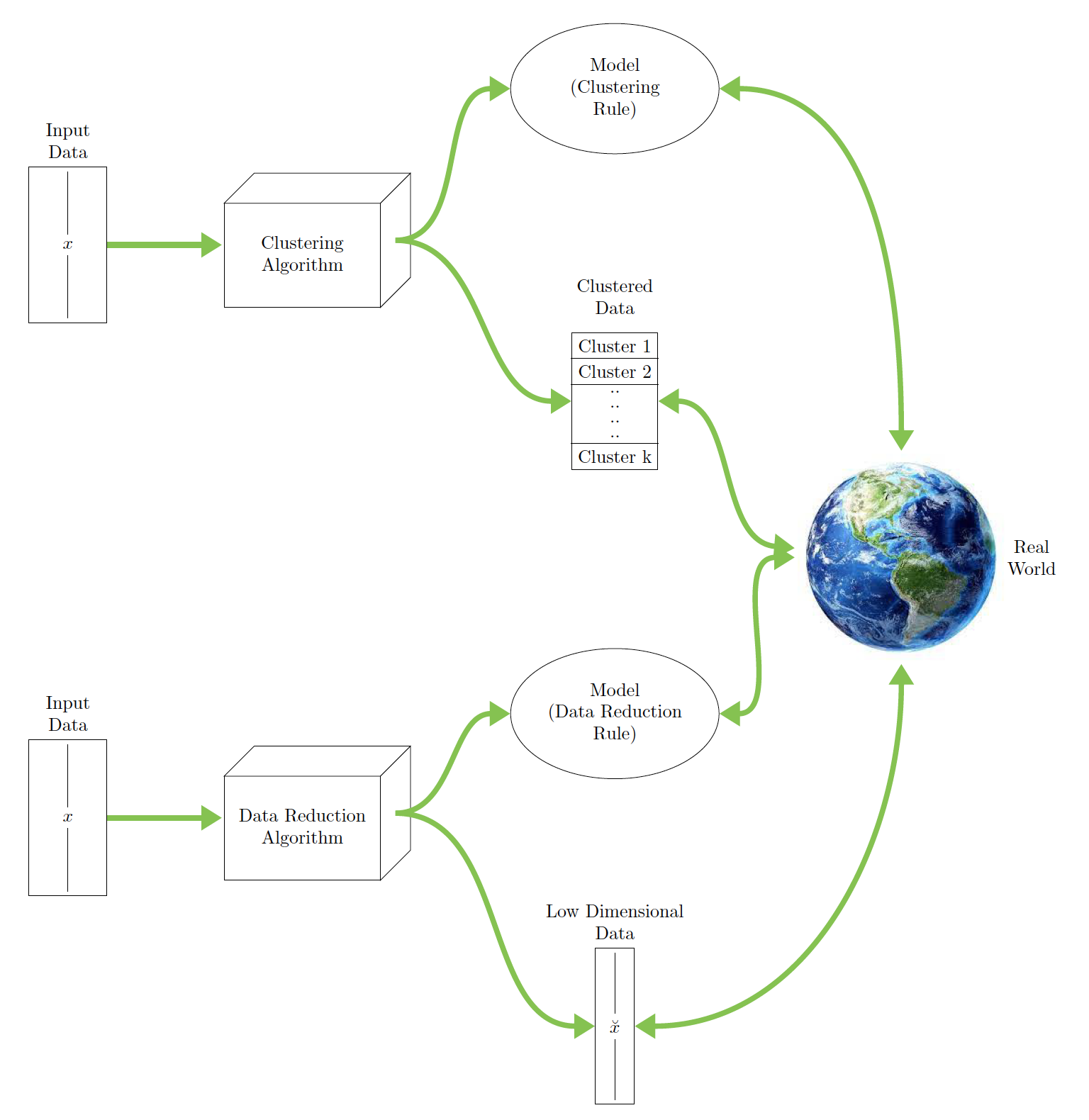
The following illustrations are taken from Chapter 2 of The Mathematical Engineering of Deep Learning. They serve to illustrate how models, algorithms, and data can interact in the world of machine learning.
This schematic illustrates supervised learning:
This schematic illustrates unsupervised learning with clustering and data reduction:
ML Datasets
There are some datasets used in machine learning learning, exploration, and (sometimes) practice that are very popular.
One of the most common datasets is the MNIST Digits dataset. It is composed of monochrome digits of $28 \times 28$ pixels and labels indicating each digit. There are $60,000$ digits that are called the training set and $10,000$ additional digits that are called the test set. In Julia you can access this dataset via the MLDatasets.jl package.
This is how we can load the training dataset.
using MLDatasets
train_data = MLDatasets.MNIST.traindata(Float64)

train_imgs = train_data[1]
@show typeof(train_imgs)
@show size(train_imgs)

train_labels = train_data[2]
@show typeof(train_labels);
typeof(train_imgs) = Array{Float64, 3}
size(train_imgs) = (28, 28, 60000)
typeof(train_labels) = Vector{Int64}
This is how we can load the testing dataset.
test_data = MLDatasets.MNIST.testdata(Float64)
test_imgs = test_data[1]
test_labels = test_data[2]
@show size(test_imgs);
size(test_imgs) = (28, 28, 10000)
Let's also keep variables for the total number of samples/observations in the training and testing dataset.
n_train, n_test = length(train_labels), length(test_labels)
(60000, 10000)
We can plot a few example training images, just to get a feel for what they look like.
using Plots, Measures, LaTeXStrings
println("The first 12 digits: ", train_labels[1:12])
plot([heatmap(train_data[1][:,:,k]',
            yflip=true,legend=false,c=cgrad([:black, :white])) for k in 1:12]...)
The first 12 digits: [5, 0, 4, 1, 9, 2, 1, 3, 1, 4, 3, 5]

It is sometimes useful to "compactify" each image into a vector. This then yields a matrix of $60,000 \times 784$ (each image has $784$ features since $784 = 28 \times 28$. Just for the heck of it, we can plot that matrix as well.
X = vcat([vec(train_imgs[:,:,k])' for k in 1:n_train]...)
@show size(X)
heatmap(X, legend=false)
size(X) = (60000, 784)

Although this looks a bit random, we can detect some trends in the pattern visually if we sort the labels first:
X_sorted = vcat([vec(train_imgs[:,:,k])' for k in sortperm(train_labels)]...)
heatmap(X_sorted, legend=false)

The data is now sorted into vertical "bands" of the digits $0, 1, \dots, 9$. MNIST is a balanced dataset, meaning that each of the digits appears about the same number of times. It is not inconceivable that a computer could be able to determine to which segment a given piece of input data belongs.
A taste of unsupervised learning
In general, unsupervised learning is the process of learning attributes of the data based only on relationships between features (pixels in the the context of images) and not based on data labels $Y$. So in unsupervised learning we only have $X$.
One type of unsupervised learning focusing on data reduction is principal component analysis (PCA). Here the data is projected from a 784-dimensional space into a smaller dimension of our choice. So for example if we choose just $2$ orthogonal basis vectors to project the above data onto, then we can "plot" each data point on this new 2D plane. Doing so and comparing some of the digits we can get a feel for how PCA can be useful.
using MultivariateStats
pca = fit(PCA, X'; maxoutdim=2)
M = projection(pca)

args = (ms=0.8, msw=0, xlims=(-5,12.5), ylims=(-7.5,7.5),
            legend = :topright, xlabel="PC 1", ylabel="PC 2")

function compareDigits(dA,dB)
    xA = X[train_labels .== dA, :]'
    xB = X[train_labels .== dB, :]'
    zA, zB = M'*xA, M'*xB

    scatter(zA[1,:], zA[2,:], c=:red, label="Digit $(dA)"; args...)
    scatter!(zB[1,:], zB[2,:], c=:blue, label="Digit $(dB)"; args...)
end

plots = []
for k in 1:5
    push!(plots,compareDigits(2k-2,2k-1))
end
plot(plots...,size = (800, 500), margin = 5mm)

With just a few more basis vectors, it might be possible to distinguish the majority of the numerals. However more complex techniques would be required to reach a high degree of accuracy.
Another common form of unsupervised learning is clustering. The goal of clustering is to find data samples that are homogenous and group them together. Within such group (or cluster) you can also find a representative data point or an average of data points in the group. This is sometimes called a centroid or centre. The most basic clustering algorithm is $k$-means. It operates by iterating the search of the centres of clusters and the data points that are in the cluster. The parameter $k$ is given before hand as the number of clusters.
Here we use the Clustering.jl package to apply $k$-means to MNIST. We then plot the resulting centroids.
using Clustering, Random
Random.seed!(0)
clusterResult = kmeans(X',10)
heatmap(hcat([reshape(clusterResult.centers[:,k],28,28)' for k in 1:10]...),
    yflip=true,legend=false,aspectratio = 1,ticks=false,c=cgrad([:black, :white]),ylim=(0,30))

Some characters are identified as quite distinct from the others, while others (like 4, 7 and 9) appear to be blended together. There are a variety of more advanced unsupervised learning algorithms that we will not cover here.
Supervised learning
A much more common form of machine learning is supervised learning where the data is comprised of the features (or independent variables) $X$ and the labels (or dependent variables or response variables) $Y$.
In cases where the variable to be predicted, $Y$, is a continuos or numerical variable, the problem is typically called a regression problem. Otherwise, in cases where $Y$ comes from some finite set of label values the problem is called a classification problem. For example in the case of MNIST digits, it is a classification problem since we need to look at an image and determine the respective digit.
Today a very popular go-to tool for supervised learning is deep learning. Other methods include tree based models, which we study in the sequel.
The basics: linear models
While not all forms of supervised learning are "deep learning", linear models are a special case of deep learning. We don't have time in this course to get into the full details of more advanced deep learning methods. But we can start with a (degenerate) neural network - a linear model.
With MNIST we can reach $86\%$ classification accuracy with a linear model. This is by no means the 99%+ accuracy that you can obtain with more advanced neural network models, but it is still an impressive measure for such a simple model. In discussing this we also explore basic aspects of classification problems.
Our data is comprised of images $x^{(1)},\ldots,x^{(n)}$ where we treat each image as $x^{(i)} \in {\mathbb R}^{784}$. There are then labels $y^{(1)},\ldots,y^{(n)}$ where $y^{(i)} \in \{0,1,2,\ldots,9\}$. For us $n=60,000$.
One approach for such multi-class classification (more than just binary classification) is to break the problem up into $10$ different binary classification problems. In each of the $10$ cases we train a classifier to classify if a digit is $0$ or not, $1$ or not, $2$ or not, etc...
If for example we train a classifier to detect $0$ or not, we set a new set of labels $\tilde{y}^{(i)}$ as $+1$ if $y^{(i)}$ is a $0$ and $-1$ if $y^{(i)}$ is not $0$. We can call this a positive sample and negative sample respectively.
To predict if a sample is positive or negative we use the basic linear model,
\[ \hat{y}^{(i)} = \beta_0 + \sum_{j=1}^{784} \beta_j x_j^{(i)}. \]
To find a "good" $\beta \in {\mathbb R}^{785}$, our aim is to minimize the quadratic loss $\big(\hat{y}^{(i)} - \tilde{y}^{(i)}\big)^2$. Summing over all observations, we have the loss function:
\[ L(\beta) = \sum_{i=1}^n \big( [1 ~~ {x^{(i)}}^\top ]^\top ~ \beta - \tilde{y}^{(i)} \big)^2. \]
Now we can define the $n\times p$ where $p=785$ design matrix which has a first column of $1$'s and the remaining columns each corresponding individual features (or pixels).
\[ A=\left[\begin{array}{ccccc} 1 & x_{1}^{(1)} & x_{2}^{(1)} & \cdots & x_{p}^{(1)} \\ 1 & x_{1}^{(2)} & x_{2}^{(2)} & \cdots & x_{p}^{(2)} \\ \vdots & \vdots & \vdots & & \vdots \\ 1 & x_{1}^{(n)} & x_{2}^{(n)} & \cdots & x_{p}^{(n)} \end{array}\right] \]
A = [ones(n_train) X];
With the matrix $A$ at hand the loss can be represented as,
\[ L(\beta) = ||A \beta - \tilde{y}||^2 = (A \beta - \tilde{y})^\top (A \beta - \tilde{y}). \]
The gradient of $L(\beta)$ is
\[ \nabla L(\beta) = 2 A^{\top}(A \beta - \tilde{y}). \]
We could use it for gradient descent (as we illustrate below) or directly equating to the $0$ vector we have the normal equations:
\[ A^\top A \beta = A^\top \tilde{y}. \]
These equations are solved via
\[ \beta = A^\dagger \tilde{y}, \]
where $A^\dagger$ is the Moore-Penrose pseudoinverse, which can be represented as $A^\dagger = (A^\top A)^{-1} A^\top$ if $A$ is skinny and full rank, but can also be computed in other cases. In any case, using the LinearAlgebra package we may obtain it via pinv():
using LinearAlgebra
Adag = pinv(A);
@show size(Adag);
size(Adag) = (785, 60000)
See also Unit 3 where we illustrated solutions of such least squares problems using multiple linear algebraic methods.
We can now find $\beta$ coefficients matching each digit. Interestingly we only need to compute the pseudo-inverse once. This is done in the code below using onehotbatch() supplied via the Flux.jl package. This function simply converts a label (0-9) to a unit vector.
using Flux: onehotbatch

tfPM(x) = x ? +1 : -1
yDat(k) = tfPM.(onehotbatch(train_labels,0:9)'[:,k+1])
bets = [Adag*yDat(k) for k in 0:9]; #this is the trained model (a list of 10 beta coeff vectors)
A binary classifier to then decide if a digit is say $0$ or not would be based on the sign (positive or negative) of the inner product of the corresponding coefficient vector in bets and $[1 ~~ {x^{(i)}}^\top ]$. If the inner product is positive the classifier would conclude it is a $0$ digit, otherwise not.
To convert such binary classifier into a multi-class classifier via a one-vs-rest approach we simply try the inner products with all $10$ coefficient vectors and choose the digit that maximizes this inner product. Here is the actual function we would use.
linear_classify(square_image) = argmax([([1 ; vec(square_image)])'*bets[k] for k in 1:10])-1
linear_classify (generic function with 1 method)
We can now try linear_classify() on the 10,000 test images. In addition to computing the accuracy, we also print the confusion matrix:
predictions = [linear_classify(test_imgs[:,:,k]) for k in 1:n_test]
confusionMatrix = [sum((predictions .== i) .& (test_labels .== j)) for i in 0:9, j in 0:9]
acc = sum(diag(confusionMatrix))/n_test

println("Accuracy: ", acc, "\nConfusion Matrix:")
show(stdout, "text/plain", confusionMatrix)
Accuracy: 0.8603
Confusion Matrix:
10×10 Matrix{Int64}:
 944     0   18    4    0   23   18    5   14   15
   0  1107   54   17   22   18   10   40   46   11
   1     2  813   23    6    3    9   16   11    2
   2     2   26  880    1   72    0    6   30   17
   2     3   15    5  881   24   22   26   27   80
   7     1    0   17    5  659   17    0   40    1
  14     5   42    9   10   23  875    1   15    1
   2     1   22   21    2   14    0  884   12   77
   7    14   37   22   11   39    7    0  759    4
   1     0    5   12   44   17    0   50   20  801
Note that with unbalanced data, accuracy is a poor performance measure. However MNIST digits are roughly balanced.
Getting a feel for gradient based learning
The type of model training we used above relied on an explicit characterization of minimizers of the loss function: solutions of the normal equations. However in more general settings such as deep neural networks, or even in the linear setting with higher dimensions, explicit solution of the first order conditions for minimization (normal equations in the case of linear models) is not possible. For this we often use iterative optimization of which the most basic form is based on first order methods that move in the direction of local best descent.
We already saw a simple example of gradient descent in Unit 3. This can work fine for small or moderate problems but in cases where there is huge data, multiple local minima, or other problems, one often uses stochastic gradient descent (SGD) or variants. As a simple illustration, the example below (approximately) optimizes a simple linear regression problem with SGD. Note that another very common which we don't show here is the use of mini-batches.
using Random, Distributions
Random.seed!(1)

n = 10^3
beta0, beta1, sigma = 2.0, 1.5, 2.5
eta = 10^-3

xVals = rand(0:0.01:5,n)
yVals = beta0 .+ beta1*xVals + rand(Normal(0,sigma),n)

pts, b = [], [0, 0]
push!(pts,b)
for k in 1:10^4
    i = rand(1:n)
    g = [   2(b[1] + b[2]*xVals[i]-yVals[i]),
            2*xVals[i]*(b[1] + b[2]*xVals[i]-yVals[i])  ]
    global b -= eta*g
    push!(pts,b)
end

p1 = plot(first.(pts),last.(pts), c=:black,lw=0.5,label="SGD path")
     scatter!([b[1]],[b[2]],c=:blue,ms=5,label="SGD")
     scatter!([beta0],[beta1],
        c=:red,ms=5,label="Actual",
        xlabel=L"\beta_0", ylabel=L"\beta_1",
        ratio=:equal, xlims=(0,2.5), ylims=(0,2.5))

p2 = scatter(xVals,yVals, c=:black, ms=1, label="Data points")
     plot!([0,5],[b[1],b[1]+5b[2]], c=:blue,label="SGD")
     plot!([0,5],[beta0,beta0+5*beta1],	c=:red, label="Actual",
            xlims=(0,5), ylims=(-5,15), xlabel = "x", ylabel = "y")

plot(p1, p2, legend=:topleft, size=(800, 400), margin = 5mm)

Logistic and Softmax Regression
While we won't focus on general deep learning networks, let us briefly see logistic regression and logistic softmax regression. These are used for binary and multi-class classification respectively and have a long tradition in statistical modeling. They are also some of the simplest non-degenerate neural networks that one can consider (see more info in Chapter 3 of The Mathematical Engineering of Deep Learning.
In a nutshell the logistic regression model is
\[ \hat{y}=\underbrace{\sigma_{\text{Sig}}\left(\overbrace{b+w^\top x}^{z}\right)}_{a}, \]
where the Sigmoid function is
\[ \label{eqn:sigmoid-in-logistic} \sigma_{\text{Sig}}(u) = \frac{1 }{1 + e^{-u}}. \]
The softmax (logistic) regression model is
\[ \hat{y}=\underbrace{S_{\text{softmax}} \big(\overbrace{b+W x}^{z\in {\mathbb R}^K}\big)}_{a\in {\mathbb R}^K}, \]
where the softmax function is,
\[ S_{\text{softmax}}(z) = \frac{1}{\sum_{i=1}^{K} e^{z_i}} \begin{bmatrix} e^{z_1} \\ \vdots\\ e^{z_{K}}\\ \end{bmatrix}. \]
The logistic regression model takes input vectors $x$ and returns probabilities (values in the range $(0,1)$). The softmax logistic regression model takes input vectors $x$ and returns probability vectors of length $K$ (probability distributions). The former can be used for binary classification and the latter for multi-class classification with $K$ classes (types to classify).
Training these models can be done for (relatively) small $x$ via the Julia package GLM.jl (Generalized Linear Models). However more generally using a deep learning framework such as Flux.jl one can handle higher dimensions of $x$ as well.
The typical loss function when training such models is called the cross entropy loss function. It measures the distance (although it isn't a proper distance metric) between two probability distributions. We skip the details.
using Flux, Statistics, Random, StatsBase, Plots
using Flux: params, onehotbatch, crossentropy, update!
Random.seed!(0)

X_test = vcat([vec(test_imgs[:,:,k])' for k in 1:n_test]...)

logistic_softmax_predict(img_vec, W, b) = softmax(W*img_vec .+ b)
logistic_sofmax_classifier(img_vec, W, b) = argmax(logistic_softmax_predict(img_vec, W, b)) - 1


function train_softmax_logistic(;mini_batch_size = 1000)

    #Initilize parameters
    W = randn(10,28*28)
    b = randn(10)

    opt = ADAM(0.01)
    loss(x, y) = crossentropy(logistic_softmax_predict(x, W, b), onehotbatch(y,0:9))

    loss_value = 0.0
    epoch_num = 0

    #Training loop
    while true
        prev_loss_value = loss_value

        #Loop over mini-batches in epoch
        start_time = time_ns()
        for batch in Iterators.partition(1:n_train, mini_batch_size)
            gs = gradient(()->loss(X'[:,batch], train_labels[batch]), params(W,b))
            for p in (W,b)
                update!(opt, p, gs[p])
            end
        end
        end_time = time_ns()

        #record/display progress
        epoch_num += 1
        loss_value = loss(X', train_labels)
        println("Epoch = $epoch_num ($(round((end_time-start_time)/1e9,digits=2)) sec) Loss = $loss_value")

        if epoch_num == 1 || epoch_num % 5 == 0
            acc = mean([logistic_sofmax_classifier(X_test'[:,k], W, b) for k in 1:n_test] .== test_labels)
            println("\tValidation accuracy: $acc")

            #Stopping criteria
            abs(prev_loss_value-loss_value) < 1e-3 && break
        end
    end
    return W, b
end

# Train model parameters
W, b = train_softmax_logistic();
Epoch = 1 (23.1 sec) Loss = 1.5558745308581823
	Validation accuracy: 0.7079
Epoch = 2 (4.58 sec) Loss = 0.9157372508918367
Epoch = 3 (4.54 sec) Loss = 0.7109639372746402
Epoch = 4 (4.44 sec) Loss = 0.6054271538755294
Epoch = 5 (4.15 sec) Loss = 0.5397156844845997
	Validation accuracy: 0.8744
Epoch = 6 (4.36 sec) Loss = 0.49402379669684787
Epoch = 7 (4.37 sec) Loss = 0.45987122954745197
Epoch = 8 (4.19 sec) Loss = 0.4330578113859848
Epoch = 9 (4.35 sec) Loss = 0.4112794620009553
Epoch = 10 (4.17 sec) Loss = 0.39316309233748165
	Validation accuracy: 0.8966
Epoch = 11 (4.32 sec) Loss = 0.37783240838239834
Epoch = 12 (4.35 sec) Loss = 0.36466710604462244
Epoch = 13 (4.22 sec) Loss = 0.3532116264199913
Epoch = 14 (4.37 sec) Loss = 0.343128181410476
Epoch = 15 (4.44 sec) Loss = 0.3341673396624744
	Validation accuracy: 0.9069
Epoch = 16 (4.12 sec) Loss = 0.3261454614467481
Epoch = 17 (4.35 sec) Loss = 0.3189246447692079
Epoch = 18 (4.38 sec) Loss = 0.3123975579557218
Epoch = 19 (4.17 sec) Loss = 0.30647805552582497
Epoch = 20 (4.36 sec) Loss = 0.30109540362712617
	Validation accuracy: 0.9108
Epoch = 21 (4.43 sec) Loss = 0.29618993864971976
Epoch = 22 (4.17 sec) Loss = 0.29170975119728415
Epoch = 23 (4.41 sec) Loss = 0.2876086869555361
Epoch = 24 (4.19 sec) Loss = 0.28384546507468833
Epoch = 25 (4.38 sec) Loss = 0.28038336148477394
	Validation accuracy: 0.915
Epoch = 26 (4.31 sec) Loss = 0.2771900038706324
Epoch = 27 (4.18 sec) Loss = 0.2742370748432038
Epoch = 28 (4.34 sec) Loss = 0.2714999021458274
Epoch = 29 (4.18 sec) Loss = 0.2689569893564704
Epoch = 30 (4.33 sec) Loss = 0.2665895480565409
	Validation accuracy: 0.9176
Epoch = 31 (4.38 sec) Loss = 0.2643810743190088
Epoch = 32 (4.16 sec) Loss = 0.2623169902234183
Epoch = 33 (4.39 sec) Loss = 0.2603843534386083
Epoch = 34 (4.37 sec) Loss = 0.25857162711740767
Epoch = 35 (4.15 sec) Loss = 0.25686849778889115
	Validation accuracy: 0.919
Epoch = 36 (4.32 sec) Loss = 0.25526572869419156
Epoch = 37 (4.41 sec) Loss = 0.2537550380830775
Epoch = 38 (4.22 sec) Loss = 0.25232899484291227
Epoch = 39 (4.33 sec) Loss = 0.2509809265238158
Epoch = 40 (4.18 sec) Loss = 0.24970483689800424
	Validation accuracy: 0.9202
Epoch = 41 (4.34 sec) Loss = 0.24849533154368103
Epoch = 42 (4.43 sec) Loss = 0.24734755068086214
Epoch = 43 (4.2 sec) Loss = 0.2462571087974986
Epoch = 44 (4.36 sec) Loss = 0.24522004067263478
Epoch = 45 (4.21 sec) Loss = 0.24423275336519903
	Validation accuracy: 0.9205
Fitting, over-fitting, generalization, and model choice
When we develop or train machine learning models we use the seen data. We often assume it is i.i.d. data and if we have reason to believe it isn't we shuffle it, or collect it in a way where it is likely to be i.i.d.
We then can choose a model to fit the data. And we want to "fit the data well". This sounds sensible, but is clearly subject to abuse. We can effectively have a model that fits every data point exactly!
Here is one example of this where our data consists of $(x,y)$ pairs and we use a Vandermonde Matrix to fit a polynomial that goes through each training point exactly. The example also has a linear fit using the pseudo-inverse. Which model is better?
As you answer this question, consider also the fact that there is unseen data which we don't get to see as we develop the model (red points in the curve).
using Plots, LinearAlgebra

x_seen = [-2, 3, 5, 6, 12, 14]
y_seen = [7, 2, 9, 3, 12, 3]
n = length(x_seen)

x_unseen = [15, -1, 5.5, 7.8]
y_unseen = [3.5, 6, 8.7, 10.4]

# Polynomial interpolation to fit exactly each point
V = [x_seen[i+1]^(j) for i in 0:n-1, j in 0:n-1]
c = V \ y_seen
f1(x) = c'*[x^i for i in 0:n-1]

#Linear fit
A = [ones(n) x_seen]
β = pinv(A)*y_seen
beta0, beta1 = 4.58, 0.17
f2(x) =β'*[1,x]

xGrid = -5:0.01:20
plot(xGrid, f1.(xGrid), c=:blue, label="Exact Polynomial fit")
plot!(xGrid, f2.(xGrid), c=:red, label="Linear model")
scatter!(x_seen, y_seen, c=:black, shape=:diamond, ms=6, label="Seen Data points")
scatter!(x_unseen, y_unseen,
    c=:red, shape=:circle, ms=6,
    label="Unseen Data points", xlims=(-5,20), ylims=(-50,50),
    xlabel = "x", ylabel = "y"
)

So in general it is obvious that a model that "fits our data exactly" is typically not the best model. Much of machine learning theory attempts to quantify this tradeoff between an over-fit of the training data and a good model. Sometimes this falls under the title of the Bias Variance tradeoff in machine learning theory where the bias of a model (or estimator) is associated with under-fitting and the variance of a model is associated with over-fitting.
We don't get into the full mathematical details of over-fitting/under-fitting, generalization error and the bias variance tradeoff. A good introductory resource for the theory of this is the book Data Science and Machine Learning: Mathematical and Statistical Methods . A much lighter book is The hundred page machine learning book.
Handling the data
In view of over-fitting and under-fitting considerations, a first thing to consider is how to handle the data. Here is an overview:
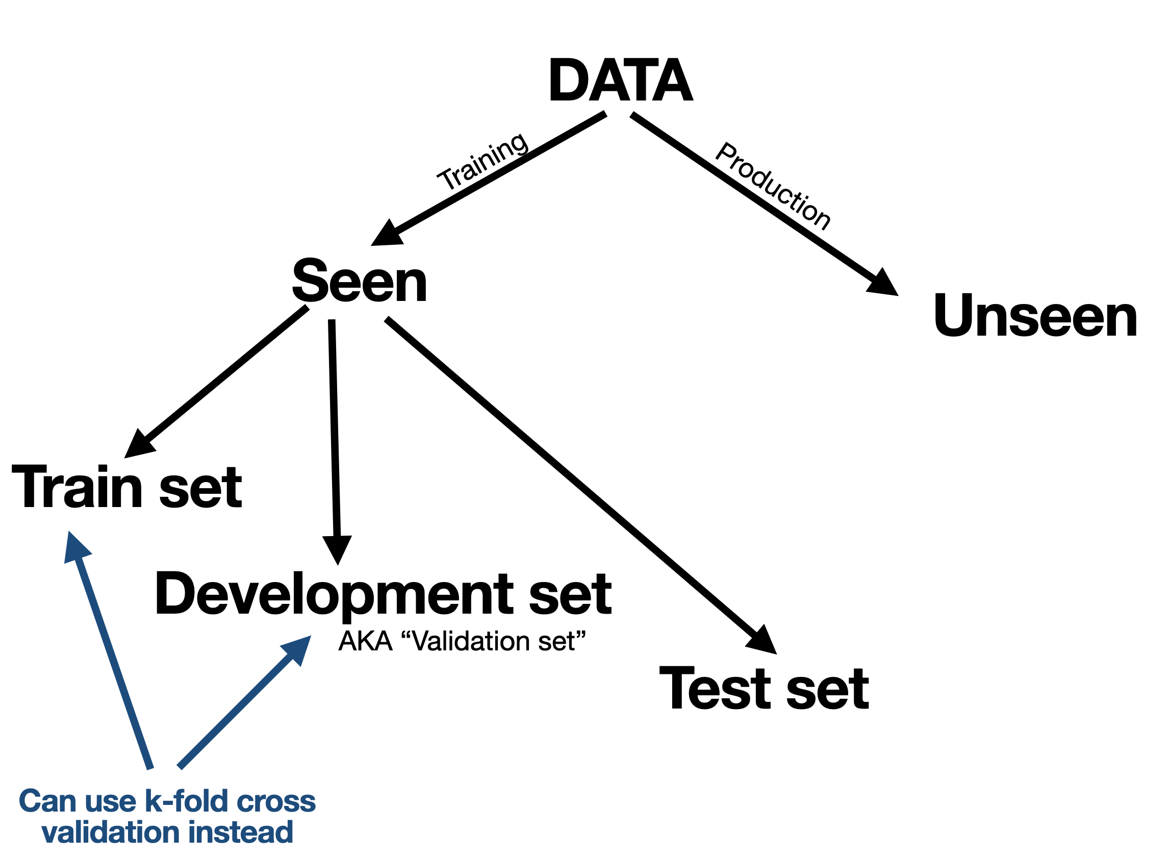
We typically split our available (seen) data into a training set and test set. The idea of the test set is to use it only once to mimic a situation where it is unseen. However the training data is further split into a training set (this word used twice) and a validation set (also known as development set) where we can tune and calibrate the model again and again on the training data while seeing how it performs on the validation set.
Sometimes instead of using a validation set we can do k-fold cross validation or some variant of it.
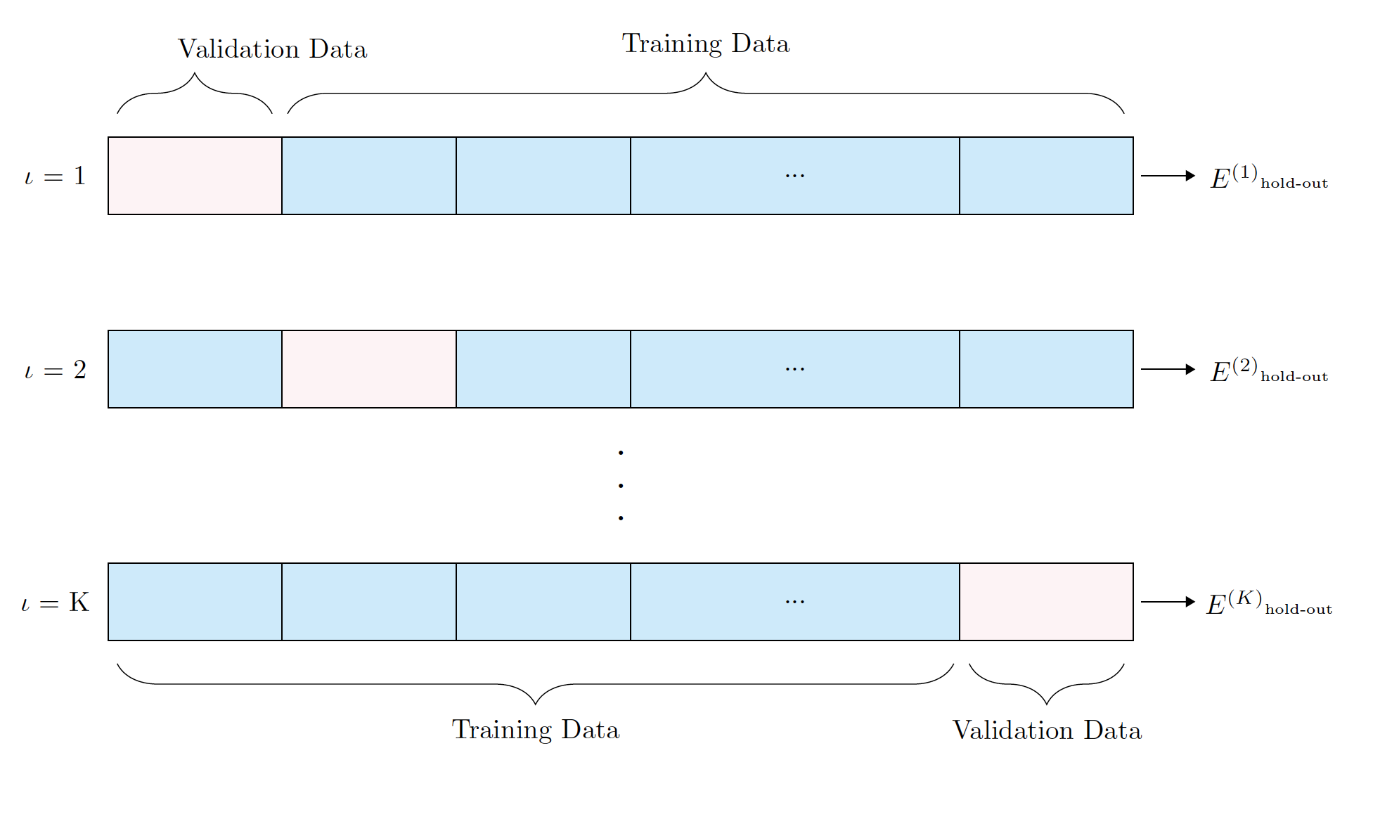
In any case, our purpose fo the training/validation/cross-validation data is to select the right model, train the model, and tune hyper-parameters.
Tree-based models
We now focus on tree-based models. Decision trees for machine learning have a long history and constitute a set of models that is still very much in use today. These models are enhanced with Random forest models which use a general machine learning technique Ensemble Method, or bagging also known as bootstrap aggregation.
We first introduce and explore basics of decision trees both for regression and classification. We then see that on their own, decision trees are somewhat limited because they can easily over-fit. We then consider random forests which constitute a much more versatile algorithm.
One of our main pedagogical reasons for focusing on tree-based models as example machine learning models in this course is simply because their programming requires using some recursive data-structures. This then provides some programming experience that is useful not just for machine learning, but also more generally.
Basic Decision trees
To illustrate we'll first consider a classification problem with $d=2$ features and $k=3$ classes. For simplicity we generate synthetic data via a mixture of bi-variate normals.
using Distributions, Random, LaTeXStrings, Plots
Random.seed!(1)

d, k = 2, 3 #d features and k label types

function make_data(class1 = 50, class2 = 30, class3 = 20)
    return (#X
            vcat(   rand(MvNormal([1,1],[3 0.7; 0.7 3]), class1)',
                    rand(MvNormal([4,2],[2.5 -0.7; -0.7 2.5]), class2)',
                    rand(MvNormal([2,4],[2 0.7; 0.7 2]), class3)')
            ,
            #y
            vcat(fill(1,class1), fill(2,class2), fill(3,class3))
            )
end

X, y = make_data()
n = length(y)
label_colors = [:red :green :blue]
xlim, ylim = (-3,8),(-3,8)

#We'll plot points again below, so putting it in in a function
function plot_points(plt_function, X, y)
    plt_function(X[:,1], X[:,2], c = label_colors, ms = 5,
        group = y, label=hcat(["class $k" for k in 1:3]...), xlabel = L"X_1", ylabel = L"X_2",
        xlim = xlim, ylim = ylim, legend = :topleft
    )
end

plot_points(scatter, X, y)

A decision-tree classifier splits the input space (in this case $\mathbb{R}^2$) into disjoint regions based on a sequence of decision rules. We illustrate this directly using code. For example, a node in such a decision tree can be implemented with nodes such as:
abstract type AbstractDecisionNode end

mutable struct DecisionNode <: AbstractDecisionNode
    # Cutoff logic
    feature::Int
    cutoff::Float64

    # Children - either another decision node or an value (label)
    lchild::Union{DecisionNode, Int64}
    rchild::Union{DecisionNode, Int64}
end
A show function is useful to have.
function Base.show(io::IO, node::AbstractDecisionNode, this_prefix = "", subtree_prefix = "")
    println(io, "$(this_prefix)─┬ feature[$(node.feature)] < $(node.cutoff)")

    # print children
    if node.lchild isa AbstractDecisionNode
        show(io, node.lchild, "$(subtree_prefix) ├", "$(subtree_prefix) │")
    else
        println(io, "$(subtree_prefix) ├── $(node.lchild)")
    end

    if node.rchild isa AbstractDecisionNode
        show(io, node.rchild, "$(subtree_prefix) └", "$(subtree_prefix)  ")
    else
        println(io, "$(subtree_prefix) └── $(node.rchild)")
    end
end
Lets first manually construct such a tree with (somewhat) arbitrary cut-offs, starting at first with a single decision based on $X_1$:
manual_tree = DecisionNode(
    1,   # 1st feature
    2.0, # Cutoff 2.0
    1,   # Left child is `1`
    2,   # Right child is `2`
)
─┬ feature[1] < 2.0
 ├── 1
 └── 2
Now prediction can be done by recursively running down the tree:
# Prediction on a node uses the cutoff
function predict(node::AbstractDecisionNode, features::Vector{Float64})
    if features[node.feature] <= node.cutoff
        return predict(node.lchild, features)
    else
        return predict(node.rchild, features)
    end
end;

# This stops when the node lchild or rchild is a value (Int64) and then prediction
predict(leaf::Int64, ::Vector{Float64}) = leaf;
Here is our (simple) tree's prediction visually:
function tree_accuracy(tree, X, y)
    return mean(predict(tree, X[i,:]) == y[i] for i in 1:size(X)[1])
end

x1_grid = xlim[1]:0.005:xlim[2]
x2_grid = ylim[1]:0.005:ylim[2]
ccol = cgrad([RGB(1,0,0), RGB(0,1,0), RGB(0,0,1)])

function plot_decision(tree, X, y)
    contour(x1_grid, x2_grid, (x1, x2) -> predict(tree, [x1, x2]),
            f = true, nlev = 3, c = ccol, legend = :none,
            title = "Training Accuracy = $(tree_accuracy(tree, X, y))")
    plot_points(scatter!, X, y)
end

plot_decision(manual_tree, X, y)

Now we can add more rules by adding more nodes (let's still do this manually):
#Split the right child
manual_tree.rchild = DecisionNode(
    2,
    4.0,
    2,
    3
)

manual_tree
─┬ feature[1] < 2.0
 ├── 1
 └─┬ feature[2] < 4.0
   ├── 2
   └── 3
plot_decision(manual_tree, X, y)

Here is one more rule:
#split the left child
manual_tree.lchild = DecisionNode(
    2,
    1.9,
    1,
    3
)
manual_tree
─┬ feature[1] < 2.0
 ├─┬ feature[2] < 1.9
 │ ├── 1
 │ └── 3
 └─┬ feature[2] < 4.0
   ├── 2
   └── 3
plot_decision(manual_tree, X, y)

You can now see that with more and more additions to the tree the training accuracy can increase since in principle, each observation can eventually lie in the correct spot. However be careful we are over-fitting!. You can in principle mitigate over-fitting by finding the right balance for how deep a tree should be using for example cross validation. But below, we'll use a more general technique called random forests.
Still, before we deal with random forests that improve accuracy and allow to mitigate over-fitting, lets see one way to build the decision tree. There are multiple ways and methods, we will focus on one method based on a greedy algorithm. This is sometimes called a "top-down" construction.
For this we'll use a slightly different struct for each node that doesn't only keep the decision rule, but also keeps the data available up to that node. We'll also keep the depth of the node in each node.
#This is meant for leafs
mutable struct DecisionWithData
    # The data available to the leaf
    X::Matrix{Float64}
    y::Vector{Int}

    # The current class of the leaf.
    value::Int64
end

#This is meant for nodes that are NOT leafs
mutable struct DecisionNodeWithData <: AbstractDecisionNode
    # The data available to the node
    X::Matrix{Float64}
    y::Vector{Int64}

    # Cutoff logic
    feature::Int64
    cutoff::Float64

    # Children - either another decision node
    lchild::Union{DecisionNodeWithData, DecisionWithData}
    rchild::Union{DecisionNodeWithData, DecisionWithData}
end

Base.show(io::IO, leaf::DecisionWithData) = Base.show(io, leaf.value)
predict(leaf::DecisionWithData, ::Vector{Float64}) = leaf.value
predict (generic function with 3 methods)
# make an empty tree
initial_tree(X, y) = DecisionWithData(X, y, 1);
auto_split_tree = initial_tree(X, y)
1
Now this splitting rule function is the most important function since it takes a node and decides how to split it. Here decision tree algorithms could use different measures, sometimes called impurity functions. In our case (and so far focusing on classification) we'll decide to split based on the feature and value that minimizes.
\[ \frac{1}{\text{num left}} \sum_{\text{left}} {\mathbf 1}\{ \text{mismatch in prediction} \} + \frac{1}{\text{num right}} \sum_{\text{right}} {\mathbf 1}\{ \text{mismatch in prediction} \}. \]
using StatsBase: mode #used here for finding the most common label

function find_splitting_rule(leaf::DecisionWithData)
    X, y = leaf.X, leaf.y
    n, d = size(X)

    loss, τ, feature = Inf, NaN, -1
    pred_left_choice, pred_right_choice = -1, -1
    final_left_bits = BitVector()

    #Loop over all features
    for j = 1:d
        #Loop over all observations
        for i in 1:n
            τ_candidate = X[i,j]
            left_bits = X[:,j] .≤ τ_candidate
            right_bits = .!left_bits
            pred_left, pred_right = 0, 0

            (sum(left_bits) == 0 || sum(left_bits) == n) && continue

            pred_left = mode(y[left_bits])
            pred_right = mode(y[right_bits])
            new_loss = mean(y[left_bits] .!= pred_left) + mean(y[right_bits] .!= pred_right)

            #if found a better split than previously then retain it
            if new_loss < loss
                final_left_bits = left_bits
                pred_left_choice = pred_left
                pred_right_choice = pred_right
                feature = j
                τ = τ_candidate
                loss = new_loss
            end
        end
    end

    return (
        feature = feature,
        cutoff = τ,
        left_value = pred_left_choice,
        right_value = pred_right_choice,
        left_bits = final_left_bits
    )
end;
We can then do this recursively. But careful if max_depth is infinity` then this is a seriously over-fitted tree because it exactly describes the the training data:
function build_tree(leaf::DecisionWithData; max_depth = Inf, depth = 0)
    length(leaf.y) == 1 && return leaf
    length(unique(leaf.y)) ≤ 1 && return leaf
    (depth ≥ max_depth) && return leaf

    splitting_result = find_splitting_rule(leaf)
    right_bits = .!splitting_result.left_bits #.! flips the bits

    lchild = build_tree(
        DecisionWithData(
            leaf.X[splitting_result.left_bits,:],
            leaf.y[splitting_result.left_bits],
            splitting_result.left_value,
        ); max_depth = max_depth, depth = depth + 1
    )

    rchild =  build_tree(
        DecisionWithData(
            leaf.X[right_bits,:],
            leaf.y[right_bits],
            splitting_result.right_value,
        ); max_depth = max_depth, depth = depth + 1
    )

    return DecisionNodeWithData(
        leaf.X,
        leaf.y,
        splitting_result.feature,
        splitting_result.cutoff,
        lchild,
        rchild
    )
end;
Let's build a tree:
auto_split_tree = build_tree(initial_tree(X, y))
plot_decision(auto_split_tree, X, y)

Let's count how many nodes we have (this is called "walking the tree"):
num_nodes(leaf::DecisionWithData) = 1
function num_nodes(node::DecisionNodeWithData)
    return 1 + num_nodes(node.lchild) + num_nodes(node.rchild)
end
num_nodes(auto_split_tree)
155
Similarly we can look at the depth of the tree (this implementation use the fact here that every node has a depth field):
depth(leaf::DecisionWithData) = 1
function depth(node::DecisionNodeWithData; max_depth = 1)
    return 1 + max(depth(node.lchild), depth(node.rchild))
end
depth(auto_split_tree)
78
Instead lets incrementally build trees with more depth
for d = 2:100
    tree = build_tree(initial_tree(X, y), max_depth = d)
    tree_summary = (
        max_depth = d,
        actual_depth = depth(tree),
        num_nodes = num_nodes(tree),
        accuracy = tree_accuracy(tree, X, y)
    )
    println(tree_summary)
end
(max_depth = 2, actual_depth = 3, num_nodes = 5, accuracy = 0.6)
(max_depth = 3, actual_depth = 4, num_nodes = 7, accuracy = 0.62)
(max_depth = 4, actual_depth = 5, num_nodes = 9, accuracy = 0.65)
(max_depth = 5, actual_depth = 6, num_nodes = 11, accuracy = 0.66)
(max_depth = 6, actual_depth = 7, num_nodes = 13, accuracy = 0.67)
(max_depth = 7, actual_depth = 8, num_nodes = 15, accuracy = 0.69)
(max_depth = 8, actual_depth = 9, num_nodes = 17, accuracy = 0.69)
(max_depth = 9, actual_depth = 10, num_nodes = 19, accuracy = 0.69)
(max_depth = 10, actual_depth = 11, num_nodes = 21, accuracy = 0.69)
(max_depth = 11, actual_depth = 12, num_nodes = 23, accuracy = 0.69)
(max_depth = 12, actual_depth = 13, num_nodes = 25, accuracy = 0.69)
(max_depth = 13, actual_depth = 14, num_nodes = 27, accuracy = 0.7)
(max_depth = 14, actual_depth = 15, num_nodes = 29, accuracy = 0.7)
(max_depth = 15, actual_depth = 16, num_nodes = 31, accuracy = 0.7)
(max_depth = 16, actual_depth = 17, num_nodes = 33, accuracy = 0.7)
(max_depth = 17, actual_depth = 18, num_nodes = 35, accuracy = 0.7)
(max_depth = 18, actual_depth = 19, num_nodes = 37, accuracy = 0.7)
(max_depth = 19, actual_depth = 20, num_nodes = 39, accuracy = 0.7)
(max_depth = 20, actual_depth = 21, num_nodes = 41, accuracy = 0.7)
(max_depth = 21, actual_depth = 22, num_nodes = 43, accuracy = 0.7)
(max_depth = 22, actual_depth = 23, num_nodes = 45, accuracy = 0.7)
(max_depth = 23, actual_depth = 24, num_nodes = 47, accuracy = 0.7)
(max_depth = 24, actual_depth = 25, num_nodes = 49, accuracy = 0.7)
(max_depth = 25, actual_depth = 26, num_nodes = 51, accuracy = 0.7)
(max_depth = 26, actual_depth = 27, num_nodes = 53, accuracy = 0.7)
(max_depth = 27, actual_depth = 28, num_nodes = 55, accuracy = 0.71)
(max_depth = 28, actual_depth = 29, num_nodes = 57, accuracy = 0.71)
(max_depth = 29, actual_depth = 30, num_nodes = 59, accuracy = 0.71)
(max_depth = 30, actual_depth = 31, num_nodes = 61, accuracy = 0.71)
(max_depth = 31, actual_depth = 32, num_nodes = 63, accuracy = 0.71)
(max_depth = 32, actual_depth = 33, num_nodes = 65, accuracy = 0.72)
(max_depth = 33, actual_depth = 34, num_nodes = 67, accuracy = 0.72)
(max_depth = 34, actual_depth = 35, num_nodes = 69, accuracy = 0.72)
(max_depth = 35, actual_depth = 36, num_nodes = 71, accuracy = 0.73)
(max_depth = 36, actual_depth = 37, num_nodes = 73, accuracy = 0.73)
(max_depth = 37, actual_depth = 38, num_nodes = 75, accuracy = 0.73)
(max_depth = 38, actual_depth = 39, num_nodes = 77, accuracy = 0.73)
(max_depth = 39, actual_depth = 40, num_nodes = 79, accuracy = 0.74)
(max_depth = 40, actual_depth = 41, num_nodes = 81, accuracy = 0.74)
(max_depth = 41, actual_depth = 42, num_nodes = 83, accuracy = 0.74)
(max_depth = 42, actual_depth = 43, num_nodes = 85, accuracy = 0.75)
(max_depth = 43, actual_depth = 44, num_nodes = 87, accuracy = 0.75)
(max_depth = 44, actual_depth = 45, num_nodes = 89, accuracy = 0.75)
(max_depth = 45, actual_depth = 46, num_nodes = 91, accuracy = 0.76)
(max_depth = 46, actual_depth = 47, num_nodes = 93, accuracy = 0.76)
(max_depth = 47, actual_depth = 48, num_nodes = 95, accuracy = 0.76)
(max_depth = 48, actual_depth = 49, num_nodes = 97, accuracy = 0.78)
(max_depth = 49, actual_depth = 50, num_nodes = 99, accuracy = 0.79)
(max_depth = 50, actual_depth = 51, num_nodes = 101, accuracy = 0.8)
(max_depth = 51, actual_depth = 52, num_nodes = 103, accuracy = 0.82)
(max_depth = 52, actual_depth = 53, num_nodes = 105, accuracy = 0.82)
(max_depth = 53, actual_depth = 54, num_nodes = 107, accuracy = 0.83)
(max_depth = 54, actual_depth = 55, num_nodes = 109, accuracy = 0.83)
(max_depth = 55, actual_depth = 56, num_nodes = 111, accuracy = 0.83)
(max_depth = 56, actual_depth = 57, num_nodes = 113, accuracy = 0.86)
(max_depth = 57, actual_depth = 58, num_nodes = 115, accuracy = 0.87)
(max_depth = 58, actual_depth = 59, num_nodes = 117, accuracy = 0.87)
(max_depth = 59, actual_depth = 60, num_nodes = 119, accuracy = 0.87)
(max_depth = 60, actual_depth = 61, num_nodes = 121, accuracy = 0.87)
(max_depth = 61, actual_depth = 62, num_nodes = 123, accuracy = 0.88)
(max_depth = 62, actual_depth = 63, num_nodes = 125, accuracy = 0.88)
(max_depth = 63, actual_depth = 64, num_nodes = 127, accuracy = 0.89)
(max_depth = 64, actual_depth = 65, num_nodes = 129, accuracy = 0.9)
(max_depth = 65, actual_depth = 66, num_nodes = 131, accuracy = 0.93)
(max_depth = 66, actual_depth = 67, num_nodes = 133, accuracy = 0.93)
(max_depth = 67, actual_depth = 68, num_nodes = 135, accuracy = 0.94)
(max_depth = 68, actual_depth = 69, num_nodes = 137, accuracy = 0.94)
(max_depth = 69, actual_depth = 70, num_nodes = 139, accuracy = 0.94)
(max_depth = 70, actual_depth = 71, num_nodes = 141, accuracy = 0.96)
(max_depth = 71, actual_depth = 72, num_nodes = 143, accuracy = 0.97)
(max_depth = 72, actual_depth = 73, num_nodes = 145, accuracy = 0.97)
(max_depth = 73, actual_depth = 74, num_nodes = 147, accuracy = 0.98)
(max_depth = 74, actual_depth = 75, num_nodes = 149, accuracy = 0.98)
(max_depth = 75, actual_depth = 76, num_nodes = 151, accuracy = 0.99)
(max_depth = 76, actual_depth = 77, num_nodes = 153, accuracy = 0.99)
(max_depth = 77, actual_depth = 78, num_nodes = 155, accuracy = 1.0)
(max_depth = 78, actual_depth = 78, num_nodes = 155, accuracy = 1.0)
(max_depth = 79, actual_depth = 78, num_nodes = 155, accuracy = 1.0)
(max_depth = 80, actual_depth = 78, num_nodes = 155, accuracy = 1.0)
(max_depth = 81, actual_depth = 78, num_nodes = 155, accuracy = 1.0)
(max_depth = 82, actual_depth = 78, num_nodes = 155, accuracy = 1.0)
(max_depth = 83, actual_depth = 78, num_nodes = 155, accuracy = 1.0)
(max_depth = 84, actual_depth = 78, num_nodes = 155, accuracy = 1.0)
(max_depth = 85, actual_depth = 78, num_nodes = 155, accuracy = 1.0)
(max_depth = 86, actual_depth = 78, num_nodes = 155, accuracy = 1.0)
(max_depth = 87, actual_depth = 78, num_nodes = 155, accuracy = 1.0)
(max_depth = 88, actual_depth = 78, num_nodes = 155, accuracy = 1.0)
(max_depth = 89, actual_depth = 78, num_nodes = 155, accuracy = 1.0)
(max_depth = 90, actual_depth = 78, num_nodes = 155, accuracy = 1.0)
(max_depth = 91, actual_depth = 78, num_nodes = 155, accuracy = 1.0)
(max_depth = 92, actual_depth = 78, num_nodes = 155, accuracy = 1.0)
(max_depth = 93, actual_depth = 78, num_nodes = 155, accuracy = 1.0)
(max_depth = 94, actual_depth = 78, num_nodes = 155, accuracy = 1.0)
(max_depth = 95, actual_depth = 78, num_nodes = 155, accuracy = 1.0)
(max_depth = 96, actual_depth = 78, num_nodes = 155, accuracy = 1.0)
(max_depth = 97, actual_depth = 78, num_nodes = 155, accuracy = 1.0)
(max_depth = 98, actual_depth = 78, num_nodes = 155, accuracy = 1.0)
(max_depth = 99, actual_depth = 78, num_nodes = 155, accuracy = 1.0)
(max_depth = 100, actual_depth = 78, num_nodes = 155, accuracy = 1.0)
Here is an animation of this:
anim = Animation()
for d in union(2:3,10:5:80)
    tree = build_tree(initial_tree(X, y), max_depth = d)
    plot_decision(tree, X, y)
    frame(anim)
end

gif(anim, "decision_tree.gif", fps = 1)

Now such over-fitting is obviously not good. Let's consider (an hypothetical) validation dataset in addition to the training dataset.
Random.seed!(1)
X, y = make_data(100,100,100) #training dataset
X_validate, y_validate = make_data(40,40,40)

p_train = plot_points(scatter, X, y)
          plot!(p_train, title = "Training data")
p_validate = plot_points(scatter, X_validate, y_validate)
          plot!(p_validate, title = "Validation data")
plot(p_train, p_validate)

By construction, the validation data above seems similar to the training data, however as we can see fitting a decision tree with a depth of more than about $10$ decreases validation accuracy. We are over-fitting!
train_accuracy = Float64[]
validation_accuracy = Float64[]

for d = 2:150
    tree = build_tree(initial_tree(X, y), max_depth = d)
    push!(train_accuracy, tree_accuracy(tree, X, y))
    push!(validation_accuracy, tree_accuracy(tree, X_validate, y_validate))
end

plot(2:150, [train_accuracy validation_accuracy],
    label = ["training" "validation"],
    ylim =(0, 1.1), legend = :bottomleft, shape = :circle,
    xlabel = "Max Depth", ylabel = "Accuracy")

Trees for regression
You can use decision trees for regression instead of classification. The key idea is to use a loss that quantifies the regression error at every split. Here typically we would need a stopping rule for how deep to go.
Dealing with categorical features
When we deal with categorical features the typical thing to do is one hot encoding. That is, if there is a categorical features with say three possible values, we will create three binary columns for this categorical feature where in each row, there is only a single $1$ in one of these columns and the other two will be $0$.
Using a package
Now that we understood the basics of decision trees, lets use a package with more versatile and optimized code. We'll use DecisionTree.jl. Another popular package is XGBoost.jl which wraps the popular XGBoost library code. In any case, when working with machine learning with Julia you will often use a framework such as MLJ. Similarly in Python the most popular choice is scikit-learn. Note that Julia also has the adapted, ScikitLearn.jl. We won't use these but rather create code directly or use DecisionTree.jl.
Back to MNIST:
y_train = train_labels
y_test = test_labels

X_train = vcat([vec(train_imgs[:,:,k])' for k in 1:n_train]...)
X_test = vcat([vec(test_imgs[:,:,k])' for k in 1:n_test]...);

size(X_train), size(X_test)
((60000, 784), (10000, 784))
Let's build a tree using the default API of DecisionTree.jl:
using DecisionTree, Statistics

# set of classification parameters and respective default values
# pruning_purity: purity threshold used for post-pruning (default: 1.0, no pruning)
# max_depth: maximum depth of the decision tree (default: -1, no maximum)
# min_samples_leaf: the minimum number of samples each leaf needs to have (default: 1)
# min_samples_split: the minimum number of samples in needed for a split (default: 2)
# min_purity_increase: minimum purity needed for a split (default: 0.0)
# n_subfeatures: number of features to select at random (default: 0, keep all)
# keyword rng: the random number generator or seed to use (default Random.GLOBAL_RNG)
n_subfeatures=0; max_depth=-1; min_samples_leaf=1; min_samples_split=2
min_purity_increase=0.0; pruning_purity = 1.0; seed=3

tree_model    =   DecisionTree.build_tree(y_train, X_train,
                        n_subfeatures,
                        max_depth,
                        min_samples_leaf,
                        min_samples_split,
                        min_purity_increase;
                        rng = seed)
Decision Tree
Leaves: 3327
Depth:  22
predicted_labels = DecisionTree.apply_tree(tree_model, X_test)
accuracy = mean(predicted_labels .== y_test)
println("\nPrediction accuracy (measured on test set of size $n_test): ",accuracy)
Prediction accuracy (measured on test set of size 10000): 0.886
Random forests
The idea of the random forest algorithm is to build an ensemble of trees, not just one tree. It builds on a more general idea studied in machine learning theory called "bagging". (There is also an idea of "boosting" that we don't discuss here). The general idea of bagging is to create an ensemble model,
\[ \hat{f}(x) = \frac{1}{b} \sum_{i=1}^b \hat{f}_i(x), \]
where each $\hat{f}_i(\cdot)$ is a model trained on a random subset of the data. The way the random subset is selected is by choosing random observations from the data with replacement. So the data used to train each $\hat{f}_i(\cdot)$ is the original data, but typically with some observations missing and some observations repeated. This randomization yields better performance.
The above averaging is for regression models and in classification a majority vote can be taken.
Random forests use the idea of bagging but also go beyond it: Each time that a decision tree $\hat{f}_i(\cdot)$ is trained, it isn't only trained on bagged observations, but is also trained with only a small random set of features available. It is typical (and has some supporting theory) to choose $\sqrt{d}$ random features in cases where there are $d$ features available.
So if the data available for training is the the vector $y$ and the $n\times d$ matrix $X$, then in a random forest each tree is trained with some random $n \times \lceil \sqrt{d}\rceil$ matrix $\tilde{X}$ which has rows randomly selected from the original $X$ with repetitions, and columns selected randomly from the original $X$ as well. The combination of many (or several) such trees then yields better prediction performance without danger of over-fitting.
Without getting into all the details, here is the heart of the random forest implementation (for classification) taken from DecisionTree.jl. This is from the file https://github.com/bensadeghi/DecisionTree.jl/blob/master/src/classification/main.jl. Note that the build_tree function already implements selecting a random features.
This is also an example to see some multi-threaded code. A concept we completely didn't discuss in this course:
function build_forest(
        labels              :: AbstractVector{T},
        features            :: AbstractMatrix{S},
        n_subfeatures       = -1,
        n_trees             = 10,
        partial_sampling    = 0.7,
        max_depth           = -1,
        min_samples_leaf    = 1,
        min_samples_split   = 2,
        min_purity_increase = 0.0;
        rng                 = Random.GLOBAL_RNG) where {S, T}

    if n_trees < 1
        throw("the number of trees must be >= 1")
    end
    if !(0.0 < partial_sampling <= 1.0)
        throw("partial_sampling must be in the range (0,1]")
    end

    if n_subfeatures == -1
        n_features = size(features, 2)
        n_subfeatures = round(Int, sqrt(n_features))
    end

    t_samples = length(labels)
    n_samples = floor(Int, partial_sampling * t_samples)

    forest = Vector{LeafOrNode{S, T}}(undef, n_trees)

    entropy_terms = util.compute_entropy_terms(n_samples)
    loss = (ns, n) -> util.entropy(ns, n, entropy_terms)

    if rng isa Random.AbstractRNG
        Threads.@threads for i in 1:n_trees
            inds = rand(rng, 1:t_samples, n_samples)
            forest[i] = build_tree(
                labels[inds],
                features[inds,:],
                n_subfeatures,
                max_depth,
                min_samples_leaf,
                min_samples_split,
                min_purity_increase,
                loss = loss,
                rng = rng)
        end
    elseif rng isa Integer # each thread gets its own seeded rng
        Threads.@threads for i in 1:n_trees
            Random.seed!(rng + i)
            inds = rand(1:t_samples, n_samples)
            forest[i] = build_tree(
                labels[inds],
                features[inds,:],
                n_subfeatures,
                max_depth,
                min_samples_leaf,
                min_samples_split,
                min_purity_increase,
                loss = loss)
        end
    else
        throw("rng must of be type Integer or Random.AbstractRNG")
    end

    return Ensemble{S, T}(forest)
end

function apply_forest(forest::Ensemble{S, T}, features::AbstractVector{S}) where {S, T}
    n_trees = length(forest)
    votes = Array{T}(undef, n_trees)
    for i in 1:n_trees
        votes[i] = apply_tree(forest.trees[i], features)
    end

    if T <: Float64
        return mean(votes)
    else
        return majority_vote(votes)
    end
end
With this, we have touched only the tip of the iceberg in terms of machine learning models. However we hope it is clear that the software component of machine learning is a central one: executing machine learning effectively requires solid coding skills. Other aspects dealing with the mathematics of machine learning can be learned in STAT3006, STAT3007, and other UQ courses. Enjoy.