UQ MATH2504
Programming of Simulation, Analysis, and Learning Systems
(Semester 2 2021)
This is an OLDER SEMESTER.
Go to current semester
Note that since this page is long, the unit is continued in a second page.
Unit 7: Working with heterogenous datasets and a view towards machine learning
In this unit we learn how to deal with heterogenous datasets using data frames. We then explore basic concepts of machine learning. A deep dive into deep learning at UQ is in the STAT3007 course. Theory of machine learning (and statistical learning) is also studied in STAT3006. Other aspects of applied statistics and data analysis are studied in STAT3500. Our purpose with this unit is just to touch the tip of the iceberg on issues of data analysis and machine learning. The Julia language knowledge acquired in the previous units should help.
Databases
This course doesn't touch databases, a rich topic of its own. (Do not confuse the term database with data structures or data frames). A database is a system that stores information in an organized and flexible manner. Many databases are relational databases and this means that they are comprised of multiple data tables that are associated via relations. The most common language for dealing with such databases is SQL. It is not a general programming language but rather a language for querying, modifying, and managing databases. At UQ you can study more about databases in the INFS2200 course as well as several other more advanced courses.
We now show you an example of database and a few things you may expect from SQL.
Relations
A "relation" is a mathematical term for a set over tuples (or named tuples), and is a generalization of a function.
For example, consider the function $y = f(x)$. (The names here are $x$ and $y$). An equivalent relation $f$ can be constructed as a set of tuples of the form $(x, y)$. A particular tuple $(x, y)$ is in the relation $f$ if and only if $y = f(x)$.
Other things which are not strictly functions may be relations. For example, we can construct a relation of real numbers $(x, y)$ where $x = y^2$. Or, equivalently, $y = \pm\sqrt{x}$. Positive values of $x$ correspond to two values of $y$ (positive or negative square root). When $x$ equals zero, there is only one solution for $y$ (also zero). And for negative $x$ there are no real $y$ that satisfy the relation. Note that I say "relation" and not "function" here - functions are only a subset of relations.
Just like functions may have multiple inputs ($x = f(a, b, c)$), a relation may consist of tuples of any size (including zero!). And both functions and relations can exist over finite, discrete sets.
There are precisely two relations over tuples of size zero (i.e. $()$) - the empty relation, and the relation containing the empty tuple $()$. You can use this fact to build up a kind of boolean logic in the language of relations, where the empty relation is false and the relation containing $()$ is true.
Outside of mathematics, the kinds of relations normally modelled in databases are of the discrete, finite-sized variety. A relation over tuples $(a, b, c)$ is equivalent to table with three columns $a$, $b$ and $c$. In a strictly relational databases, the ordering of the rows is irrelevant, and you cannot have two identical rows in the database (though in practice many databases in use may also deal with "bags" rather than "sets" of tuples, where rows can be repeated). The fields $a$, $b$ and $c$ are drawn from their own set of possibilities, or datatype. For example, you might have (name, birthdate, is_adult) where name may be a string, birthdate may be a date, and is_adult may be a boolean.
name | birthdate | is_adult |
|---|---|---|
"Alice" | 2001-05-13 | true |
"Bob" | 2003-12-10 | false |
"Charlie" | 2002-09-21 | true |
Note that this particular relation is also a function, since is_adult has a functional relationship with birthdate.
In many relations, there are uniqueness constraints - for example the name might identify each row uniquely, or there may be a specific ID column to deal with different people sharing the same name. Such unique constraints are called "keys" and the primary identifier that you might use to fetch a particular row is called the "primary key".
Relational schema
A single relation is a restrictive way to model your data. However, by allowing multiple relations, we can capture the various sets of data in the system, and piece them together by their relationships.
For example, each person in the table above might be related to other things. They might have jobs, bank accounts, etc. Within a single business a person might be a customer, a supplier and an employee, and for different purposes we might want data associated with that person (e.g. their birthdate might relate to promotions for customers, payrates for employees, etc).
Generally, to make keeping track of data easy, in a relational database you would store that person just once and create relationships between that person and other things. That way, if something changes about that person, it only needs to be updated in one place, and data remains consistent everywhere.
Here is an example of a more complex example - an imagining of how LinkedIn might store their data in a relational database (taken from "Designing Data-Intensive Applications" by Martin Kleppmann).
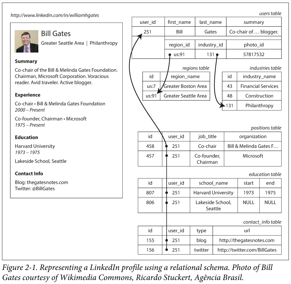
SQL
The most popular way to interact with relational data is with via a language called SQL (originally "SEQUEL", pronounced that way, backronymed to "structured query language").
The language is from 1973 and doesn't look like most other programming languages. With it, you declare a "query" and the database will find the best way to return the results. It is a form of declarative programming. Here is an example of getting some columns of data from the users table:
SELECT user_id, first_name, last_name
FROM users
You can filter the rows via a WHERE clause. Let's say you knew the user_id for Bill Gates and you wanted just his data:
SELECT user_id, first_name, last_name
FROM users
WHERE user_id = 251
Data in different tables are related via the JOIN statement
SELECT users.user_id, first_name, last_name, organization
INNER JOIN positions ON positions.user_id = users.user_id
FROM users
Note we have to prefix the shared column names with the corresponding table (although in this case the difference is not particularly important, your query cannot be ambiguous).
But there is a problem here. This query would create a large amount of data, that the database would need to collect and send over the network to you. In the worst case, performing such a query could bring down a large system!
Generally, you have something more precise in mind. Like - which organizations has Bill Gates worked at?
SELECT users.user_id, first_name, last_name, organization
INNER JOIN positions ON positions.user_id = users.user_id
FROM users
WHERE users.user_id = 251
This will now return just two rows (for Microsoft, and the Bill & Melinda Gates Foundation), and is much less effort for the database, the network and the client. In real-world settings, complex joins could link data spanning dozens of tables.
We won't be using SQL in this course but it is so pervasive in industry that is essential that you know that it exists, and not to be afraid to use it! (It is a very useful and desirable skill!).
Dataframes
Working with tabular data is a central part of data analysis (think Excel). Data has rows (observations) and columns (variables/features). Typically a row would be for an individual, or item, or event. Typically a column would be for attributes of the individual, properties of the events, etc. Variables can be numerical, categorical, strings, or even more complex entities (e.g. images, arrays or dictionaries).
The datafile athlete_events.csv is a moderately sized dataset available from Kaggle covering all athletes that have participated the Summer or Winter Olympics between 1896 and 2016. The CSV file contains 40MB of data over 15 columns and more than 27,000 rows, which is "small data" for a modern computer (but would have been challenging in the 1980's). In this context, "big data" is too large to be handled by a single machine, and we'll discuss "big data" and "medium data" later.
You have already seen how to read and write from CSV files in Unit 3 where you also explored JSON files. You may recall using the DataFrames.jl package in that unit. We now take a deeper dive into the concept of dataframes.
We will use athlete_events.csv to show basic functionality of the DataFrames.jl and TypedTables.jl packages. In a sense these packages are alternatives. Seeing some functionality from each may be useful for gaining a general understanding of what to expect from such packages. If you work with Python, then using pandas is the common alternative. Similarly if you work with the R language then the built-in dataframes are common.
Basic data exploration
Whenever you receive a dataset, it takes some time to understand its contents. This process is generally known as "data exploration". To do so, we generally load (a subset of) the data from disk and do some basic analysis in a Jupyter notebook or at the REPL.
We were introduced to CSV files earlier in the course. Here's the first few lines of our file:
open("../data/athlete_events.csv") do io
    i = 0
    while i < 5
        println(readline(io))
        i += 1
    end
end
"ID","Name","Sex","Age","Height","Weight","Team","NOC","Games","Year","Seas
on","City","Sport","Event","Medal"
"1","A Dijiang","M",24,180,80,"China","CHN","1992 Summer",1992,"Summer","Ba
rcelona","Basketball","Basketball Men's Basketball",NA
"2","A Lamusi","M",23,170,60,"China","CHN","2012 Summer",2012,"Summer","Lon
don","Judo","Judo Men's Extra-Lightweight",NA
"3","Gunnar Nielsen Aaby","M",24,NA,NA,"Denmark","DEN","1920 Summer",1920,"
Summer","Antwerpen","Football","Football Men's Football",NA
"4","Edgar Lindenau Aabye","M",34,NA,NA,"Denmark/Sweden","DEN","1900 Summer
",1900,"Summer","Paris","Tug-Of-War","Tug-Of-War Men's Tug-Of-War","Gold"
The do syntax here injects a function which takes io::IO (an I/O stream for our file) into the first argument of the open function. It is syntax sugar. The open function is designed such that when the inner function returns or throws an error, open will automatically close the file to avoid resource leakage.
We can use the CSV.jl package to read the data and the DataFrames.jl package to hold the tabular data. We note in the above the appearance of "NA" for missing data, which we can use to help load the file.
using DataFrames, CSV
csv_file = CSV.File("../data/athlete_events.csv"; missingstring = "NA")
df = DataFrame(csv_file)
println("Data size: ", size(df))
println("Columns in the data: ", names(df))
Data size: (271116, 15)
Columns in the data: ["ID", "Name", "Sex", "Age", "Height", "Weight", "Team
", "NOC", "Games", "Year", "Season", "City", "Sport", "Event", "Medal"]
Since the data is large, we don't usually want to print it all. The first and last functions can be helpful:
first(df, 10)
10 rows × 15 columns (omitted printing of 8 columns)
| ID | Name | Sex | Age | Height | Weight | Team | |
|---|---|---|---|---|---|---|---|
| Int64 | String | String1 | Int64? | Int64? | Float64? | String63 | |
| 1 | 1 | A Dijiang | M | 24 | 180 | 80.0 | China |
| 2 | 2 | A Lamusi | M | 23 | 170 | 60.0 | China |
| 3 | 3 | Gunnar Nielsen Aaby | M | 24 | missing | missing | Denmark |
| 4 | 4 | Edgar Lindenau Aabye | M | 34 | missing | missing | Denmark/Sweden |
| 5 | 5 | Christine Jacoba Aaftink | F | 21 | 185 | 82.0 | Netherlands |
| 6 | 5 | Christine Jacoba Aaftink | F | 21 | 185 | 82.0 | Netherlands |
| 7 | 5 | Christine Jacoba Aaftink | F | 25 | 185 | 82.0 | Netherlands |
| 8 | 5 | Christine Jacoba Aaftink | F | 25 | 185 | 82.0 | Netherlands |
| 9 | 5 | Christine Jacoba Aaftink | F | 27 | 185 | 82.0 | Netherlands |
| 10 | 5 | Christine Jacoba Aaftink | F | 27 | 185 | 82.0 | Netherlands |
last(df, 10)
10 rows × 15 columns (omitted printing of 8 columns)
| ID | Name | Sex | Age | Height | Weight | Team | |
|---|---|---|---|---|---|---|---|
| Int64 | String | String1 | Int64? | Int64? | Float64? | String63 | |
| 1 | 135565 | Fernando scar Zylberberg | M | 27 | 168 | 76.0 | Argentina |
| 2 | 135566 | James Francis "Jim" Zylker | M | 21 | 175 | 75.0 | United States |
| 3 | 135567 | Aleksandr Viktorovich Zyuzin | M | 24 | 183 | 72.0 | Russia |
| 4 | 135567 | Aleksandr Viktorovich Zyuzin | M | 28 | 183 | 72.0 | Russia |
| 5 | 135568 | Olga Igorevna Zyuzkova | F | 33 | 171 | 69.0 | Belarus |
| 6 | 135569 | Andrzej ya | M | 29 | 179 | 89.0 | Poland-1 |
| 7 | 135570 | Piotr ya | M | 27 | 176 | 59.0 | Poland |
| 8 | 135570 | Piotr ya | M | 27 | 176 | 59.0 | Poland |
| 9 | 135571 | Tomasz Ireneusz ya | M | 30 | 185 | 96.0 | Poland |
| 10 | 135571 | Tomasz Ireneusz ya | M | 34 | 185 | 96.0 | Poland |
This dataset appears to be sorted by last name. Each row corresponds to an entrant to an event. The ID column identifies each unique athlete.
A DataFrame is indexed like a 2D container of rows and columns. The : symbol means "all".
df[1:10, :]
10 rows × 15 columns (omitted printing of 8 columns)
| ID | Name | Sex | Age | Height | Weight | Team | |
|---|---|---|---|---|---|---|---|
| Int64 | String | String1 | Int64? | Int64? | Float64? | String63 | |
| 1 | 1 | A Dijiang | M | 24 | 180 | 80.0 | China |
| 2 | 2 | A Lamusi | M | 23 | 170 | 60.0 | China |
| 3 | 3 | Gunnar Nielsen Aaby | M | 24 | missing | missing | Denmark |
| 4 | 4 | Edgar Lindenau Aabye | M | 34 | missing | missing | Denmark/Sweden |
| 5 | 5 | Christine Jacoba Aaftink | F | 21 | 185 | 82.0 | Netherlands |
| 6 | 5 | Christine Jacoba Aaftink | F | 21 | 185 | 82.0 | Netherlands |
| 7 | 5 | Christine Jacoba Aaftink | F | 25 | 185 | 82.0 | Netherlands |
| 8 | 5 | Christine Jacoba Aaftink | F | 25 | 185 | 82.0 | Netherlands |
| 9 | 5 | Christine Jacoba Aaftink | F | 27 | 185 | 82.0 | Netherlands |
| 10 | 5 | Christine Jacoba Aaftink | F | 27 | 185 | 82.0 | Netherlands |
Internally, a dataframe stores one vector of data per column. You can access any of them conveniently as "properties" with . syntax:
df.ID
271116-element Vector{Int64}:
      1
      2
      3
      4
      5
      5
      5
      5
      5
      5
      ⋮
 135566
 135567
 135567
 135568
 135569
 135570
 135570
 135571
 135571
df.Height
271116-element Vector{Union{Missing, Int64}}:
 180
 170
    missing
    missing
 185
 185
 185
 185
 185
 185
   ⋮
 175
 183
 183
 171
 179
 176
 176
 185
 185
As you can see from above, some data can be missing. How many heights are missing?
ismissing.(df.Height) |> count # Piping: `f(x) |> g` syntax means `g(f(x))`
60171
The count function counts the number of true values.
How many unique athletes are there?
unique(df.ID) |> length
135571
The unique operation has extra methods defined for DataFrames. We can get the athlete data like so:
athlete_df = unique(df, :ID)
135,571 rows × 15 columns (omitted printing of 8 columns)
| ID | Name | Sex | Age | Height | Weight | Team | |
|---|---|---|---|---|---|---|---|
| Int64 | String | String1 | Int64? | Int64? | Float64? | String63 | |
| 1 | 1 | A Dijiang | M | 24 | 180 | 80.0 | China |
| 2 | 2 | A Lamusi | M | 23 | 170 | 60.0 | China |
| 3 | 3 | Gunnar Nielsen Aaby | M | 24 | missing | missing | Denmark |
| 4 | 4 | Edgar Lindenau Aabye | M | 34 | missing | missing | Denmark/Sweden |
| 5 | 5 | Christine Jacoba Aaftink | F | 21 | 185 | 82.0 | Netherlands |
| 6 | 6 | Per Knut Aaland | M | 31 | 188 | 75.0 | United States |
| 7 | 7 | John Aalberg | M | 31 | 183 | 72.0 | United States |
| 8 | 8 | Cornelia "Cor" Aalten (-Strannood) | F | 18 | 168 | missing | Netherlands |
| 9 | 9 | Antti Sami Aalto | M | 26 | 186 | 96.0 | Finland |
| 10 | 10 | Einar Ferdinand "Einari" Aalto | M | 26 | missing | missing | Finland |
| 11 | 11 | Jorma Ilmari Aalto | M | 22 | 182 | 76.5 | Finland |
| 12 | 12 | Jyri Tapani Aalto | M | 31 | 172 | 70.0 | Finland |
| 13 | 13 | Minna Maarit Aalto | F | 30 | 159 | 55.5 | Finland |
| 14 | 14 | Pirjo Hannele Aalto (Mattila-) | F | 32 | 171 | 65.0 | Finland |
| 15 | 15 | Arvo Ossian Aaltonen | M | 22 | missing | missing | Finland |
| 16 | 16 | Juhamatti Tapio Aaltonen | M | 28 | 184 | 85.0 | Finland |
| 17 | 17 | Paavo Johannes Aaltonen | M | 28 | 175 | 64.0 | Finland |
| 18 | 18 | Timo Antero Aaltonen | M | 31 | 189 | 130.0 | Finland |
| 19 | 19 | Win Valdemar Aaltonen | M | 54 | missing | missing | Finland |
| 20 | 20 | Kjetil Andr Aamodt | M | 20 | 176 | 85.0 | Norway |
| 21 | 21 | Ragnhild Margrethe Aamodt | F | 27 | 163 | missing | Norway |
| 22 | 22 | Andreea Aanei | F | 22 | 170 | 125.0 | Romania |
| 23 | 23 | Fritz Aanes | M | 22 | 187 | 89.0 | Norway |
| 24 | 24 | Nils Egil Aaness | M | 24 | missing | missing | Norway |
| ⋮ | ⋮ | ⋮ | ⋮ | ⋮ | ⋮ | ⋮ | ⋮ |
It keeps all columns of the first row containing each distinct ID, which will we take as representative (for their Sex, Height, Weight, etc).
Simple analysis
Now we are becoming familiar with the dataset, we might like to see what insights we can gain. For example, let's see how many men and women have competed.
count(==("M"), athlete_df.Sex) # `==(x)` creates a function `y -> y == x`
101590
count(==("F"), athlete_df.Sex)
33981
The count function is useful, but this gets tiresome for many "groups" of data. The SplitApplyCombine.jl package contains useful functions for grouping data.
using SplitApplyCombine

groupcount(athlete_df.Sex)
2-element Dictionaries.Dictionary{String1, Int64}
 "M" │ 101590
 "F" │ 33981
Which allows us to explore larger sets of groupings:
# How many athletes by country
team_sizes = groupcount(athlete_df.Team)
1013-element Dictionaries.Dictionary{String63, Int64}
          "China" │ 2589
        "Denmark" │ 1840
 "Denmark/Sweden" │ 5
    "Netherlands" │ 2849
  "United States" │ 9051
        "Finland" │ 2271
         "Norway" │ 2029
        "Romania" │ 1735
        "Estonia" │ 336
         "France" │ 5717
                ⋮ │ ⋮
       "Sjovinge" │ 2
    "Brandenburg" │ 1
        "Struten" │ 1
       "Freia-19" │ 1
   "Luxembourg-1" │ 1
      "Sea Dog-2" │ 2
          "Mainz" │ 1
        "Druzhba" │ 1
        "China-3" │ 2
One of the most powerful tricks in data analysis is to sort your data.
sort(team_sizes)
1013-element Dictionaries.Dictionary{String63, Int64}
     "Nigeria-2" │ 1
 "Puerto Rico-2" │ 1
          "Lett" │ 1
       "Breslau" │ 1
  "Carabinier-5" │ 1
      "Evita VI" │ 1
      "Konstanz" │ 1
          "Nora" │ 1
          "Inca" │ 1
         "Snude" │ 1
               ⋮ │ ⋮
        "Sweden" │ 3598
     "Australia" │ 3731
         "Japan" │ 3990
       "Germany" │ 4318
        "Canada" │ 4504
         "Italy" │ 4650
 "Great Britain" │ 5706
        "France" │ 5717
 "United States" │ 9051
Note that groupcount is a specialization of the more flexible group(keys, values) function:
group(athlete_df.Team, athlete_df.Name)
1013-element Dictionaries.Dictionary{String63, Vector{String}}
          "China" │ ["A Dijiang", "A Lamusi", "Abudoureheman", "Ai Linuer",
 "Ai…
        "Denmark" │ ["Gunnar Nielsen Aaby", "Otto Mnsted Acthon", "Jesper A
gerg…
 "Denmark/Sweden" │ ["Edgar Lindenau Aabye", "August Nilsson", "Gustaf Fred
rik …
    "Netherlands" │ ["Christine Jacoba Aaftink", "Cornelia \"Cor\" Aalten (
-Str…
  "United States" │ ["Per Knut Aaland", "John Aalberg", "Stephen Anthony Ab
as",…
        "Finland" │ ["Antti Sami Aalto", "Einar Ferdinand \"Einari\" Aalto"
, "J…
         "Norway" │ ["Kjetil Andr Aamodt", "Ragnhild Margrethe Aamodt", "Fr
itz …
        "Romania" │ ["Andreea Aanei", "Andrei Abraham", "Elisabeta Abrudean
u", …
        "Estonia" │ ["Evald rma (rman-)", "Meelis Aasme", "Moonika Aava", "
Arvi…
         "France" │ ["Jamale (Djamel-) Aarrass (Ahrass-)", "Patrick Abada",
 "Re…
                ⋮ │ ⋮
       "Sjovinge" │ ["Christian Vinge", "Bengt Gran Waller"]
    "Brandenburg" │ ["Erik Johannes Peter Ernst von Holst"]
        "Struten" │ ["Knut Astrup Wang"]
       "Freia-19" │ ["Georges Camille Warenhorst"]
   "Luxembourg-1" │ ["Gza Wertheim"]
      "Sea Dog-2" │ ["Thomas Douglas Wynn Weston", "Joseph Warwick Wright"]
          "Mainz" │ ["Erich Wichmann-Harbeck"]
        "Druzhba" │ ["Valentin Alekseyevich Zamotaykin"]
        "China-3" │ ["Zhang Dan", "Zhang Hao"]
Rather than acting at the level of vectors, you can group an entire DataFrame into a GroupedDataFrame with the groupby function provided by DataFrames.jl:
gdf = groupby(athlete_df, :Team)
GroupedDataFrame with 1013 groups based on key: Team
First Group (2589 rows): Team = "China"
| ID | Name | Sex | Age | Height | Weight | Team | NOC | Games | |
|---|---|---|---|---|---|---|---|---|---|
| Int64 | String | String1 | Int64? | Int64? | Float64? | String63 | String3 | String15 | |
| 1 | 1 | A Dijiang | M | 24 | 180 | 80.0 | China | CHN | 1992 Summer |
| 2 | 2 | A Lamusi | M | 23 | 170 | 60.0 | China | CHN | 2012 Summer |
| 3 | 602 | Abudoureheman | M | 22 | 182 | 75.0 | China | CHN | 2000 Summer |
| 4 | 1463 | Ai Linuer | M | 25 | 160 | 62.0 | China | CHN | 2004 Summer |
| 5 | 1464 | Ai Yanhan | F | 14 | 168 | 54.0 | China | CHN | 2016 Summer |
| 6 | 3605 | An Weijiang | M | 22 | 178 | 72.0 | China | CHN | 2006 Winter |
| 7 | 3610 | An Yulong | M | 19 | 173 | 70.0 | China | CHN | 1998 Winter |
| 8 | 3611 | An Zhongxin | F | 23 | 170 | 65.0 | China | CHN | 1996 Summer |
| 9 | 4639 | Ao Changrong | M | 25 | 173 | 71.0 | China | CHN | 2008 Summer |
| 10 | 4641 | Ao Tegen | M | 21 | 181 | 90.0 | China | CHN | 1996 Summer |
| 11 | 6376 | Ba Dexin | M | 23 | 185 | 80.0 | China | CHN | 2014 Winter |
| 12 | 6381 | Ba Yan | F | 21 | 183 | 78.0 | China | CHN | 1984 Summer |
| 13 | 6382 | Ba Yanchuan | M | 24 | 187 | 100.0 | China | CHN | 1996 Summer |
| 14 | 6383 | Ba Yongshan | M | 22 | 180 | 70.0 | China | CHN | 1984 Summer |
| 15 | 6847 | Bai Anqi | F | 19 | 164 | 59.0 | China | CHN | 2012 Summer |
| 16 | 6848 | Bai Chongguang | M | 21 | 184 | 83.0 | China | CHN | 1992 Summer |
| 17 | 6849 | Bai Faquan | M | 26 | 173 | 66.0 | China | CHN | 2012 Summer |
| 18 | 6851 | Bai Jie | F | 28 | 163 | 53.0 | China | CHN | 2000 Summer |
| 19 | 6853 | Bai Lili | F | 25 | 168 | 57.0 | China | CHN | 2004 Summer |
| 20 | 6854 | Bai Mei | F | 17 | 166 | 46.0 | China | CHN | 1992 Summer |
| 21 | 6855 | Bai Qiuming | M | 19 | 173 | 70.0 | China | CHN | 2014 Winter |
| 22 | 6857 | Bai Xue | F | 19 | 165 | 53.0 | China | CHN | 2008 Summer |
| 23 | 7595 | Bao Chunlai | M | 21 | 190 | 80.0 | China | CHN | 2004 Summer |
| 24 | 7596 | Bao Jiaping | M | 27 | 177 | 55.0 | China | CHN | 1936 Summer |
| ⋮ | ⋮ | ⋮ | ⋮ | ⋮ | ⋮ | ⋮ | ⋮ | ⋮ | ⋮ |
⋮
Last Group (1 row): Team = "Mainz"
| ID | Name | Sex | Age | Height | Weight | Team | NOC | |
|---|---|---|---|---|---|---|---|---|
| Int64 | String | String1 | Int64? | Int64? | Float64? | String63 | String3 | |
| 1 | 130140 | Erich Wichmann-Harbeck | M | 35 | missing | missing | Mainz | CHI |
You can apply an operation to each group and bring the data together into a single DataFrame via the combine function.
combine(gdf, nrow => :Count)
1,013 rows × 2 columns
| Team | Count | |
|---|---|---|
| String63 | Int64 | |
| 1 | China | 2589 |
| 2 | Denmark | 1840 |
| 3 | Denmark/Sweden | 5 |
| 4 | Netherlands | 2849 |
| 5 | United States | 9051 |
| 6 | Finland | 2271 |
| 7 | Norway | 2029 |
| 8 | Romania | 1735 |
| 9 | Estonia | 336 |
| 10 | France | 5717 |
| 11 | Taifun | 5 |
| 12 | Morocco | 459 |
| 13 | Spain | 2576 |
| 14 | Egypt | 974 |
| 15 | Iran | 526 |
| 16 | Bulgaria | 1487 |
| 17 | Italy | 4650 |
| 18 | Chad | 26 |
| 19 | Azerbaijan | 174 |
| 20 | Sudan | 80 |
| 21 | Russia | 2108 |
| 22 | Argentina | 1784 |
| 23 | Cuba | 1276 |
| 24 | Belarus | 716 |
| ⋮ | ⋮ | ⋮ |
The nrow => :Count syntax is a convenience provided by Dataframes.jl. We'll explain how it works below.
Row- and column-based storage
What is a dataframe?
It is a data structure containing rows and columns. Internally it keeps each column of data as its own vector, which you can access as a property with .
athlete_df.Height
135571-element Vector{Union{Missing, Int64}}:
 180
 170
    missing
    missing
 185
 188
 183
 168
 186
    missing
   ⋮
 171
 172
 168
 175
 183
 171
 179
 176
 185
To construct a row, you need to grab the corresponding element from each vector.
first(eachrow(df))
DataFrameRow (15 columns)
| ID | Name | Sex | Age | Height | Weight | Team | NOC | Games | |
|---|---|---|---|---|---|---|---|---|---|
| Int64 | String | String1 | Int64? | Int64? | Float64? | String63 | String3 | String15 | |
| 1 | 1 | A Dijiang | M | 24 | 180 | 80.0 | China | CHN | 1992 Summer |
Or, you can use 2D indexing, as before
df[1, :]
DataFrameRow (15 columns)
| ID | Name | Sex | Age | Height | Weight | Team | NOC | Games | |
|---|---|---|---|---|---|---|---|---|---|
| Int64 | String | String1 | Int64? | Int64? | Float64? | String63 | String3 | String15 | |
| 1 | 1 | A Dijiang | M | 24 | 180 | 80.0 | China | CHN | 1992 Summer |
In this case there are 15 columns, so the computer must fetch data from 15 different places. This means that, for dataframes, operating with columns is faster than with rows. DataFrames are specialized for whole-of-table analytics, where each individual step in your analysis probably only involves a small number of columns.
There are other data structures you can use which store the data as rows. Most SQL databases will store their data like this. Traditional "transactional" databases are typically driven with reads and writes to one (or a few) rows at a time, and row-based storage is more efficient for such workloads. Some of the modern "analytics" databses will use column-based storage.
In Julia, perhaps the simplest such data structure is a Vector of NamedTuples. We can create one straightforwardly from a CSV.File:
NamedTuple.(csv_file)
271116-element Vector{NamedTuple{(:ID, :Name, :Sex, :Age, :Height, :Weight,
 :Team, :NOC, :Games, :Year, :Season, :City, :Sport, :Event, :Medal), T} wh
ere T<:Tuple}:
 (ID = 1, Name = "A Dijiang", Sex = "M", Age = 24, Height = 180, Weight = 8
0.0, Team = "China", NOC = "CHN", Games = "1992 Summer", Year = 1992, Seaso
n = "Summer", City = "Barcelona", Sport = "Basketball", Event = "Basketball
 Men's Basketball", Medal = missing)
 (ID = 2, Name = "A Lamusi", Sex = "M", Age = 23, Height = 170, Weight = 60
.0, Team = "China", NOC = "CHN", Games = "2012 Summer", Year = 2012, Season
 = "Summer", City = "London", Sport = "Judo", Event = "Judo Men's Extra-Lig
htweight", Medal = missing)
 (ID = 3, Name = "Gunnar Nielsen Aaby", Sex = "M", Age = 24, Height = missi
ng, Weight = missing, Team = "Denmark", NOC = "DEN", Games = "1920 Summer",
 Year = 1920, Season = "Summer", City = "Antwerpen", Sport = "Football", Ev
ent = "Football Men's Football", Medal = missing)
 (ID = 4, Name = "Edgar Lindenau Aabye", Sex = "M", Age = 34, Height = miss
ing, Weight = missing, Team = "Denmark/Sweden", NOC = "DEN", Games = "1900
Summer", Year = 1900, Season = "Summer", City = "Paris", Sport = "Tug-Of-Wa
r", Event = "Tug-Of-War Men's Tug-Of-War", Medal = "Gold")
 (ID = 5, Name = "Christine Jacoba Aaftink", Sex = "F", Age = 21, Height =
185, Weight = 82.0, Team = "Netherlands", NOC = "NED", Games = "1988 Winter
", Year = 1988, Season = "Winter", City = "Calgary", Sport = "Speed Skating
", Event = "Speed Skating Women's 500 metres", Medal = missing)
 (ID = 5, Name = "Christine Jacoba Aaftink", Sex = "F", Age = 21, Height =
185, Weight = 82.0, Team = "Netherlands", NOC = "NED", Games = "1988 Winter
", Year = 1988, Season = "Winter", City = "Calgary", Sport = "Speed Skating
", Event = "Speed Skating Women's 1,000 metres", Medal = missing)
 (ID = 5, Name = "Christine Jacoba Aaftink", Sex = "F", Age = 25, Height =
185, Weight = 82.0, Team = "Netherlands", NOC = "NED", Games = "1992 Winter
", Year = 1992, Season = "Winter", City = "Albertville", Sport = "Speed Ska
ting", Event = "Speed Skating Women's 500 metres", Medal = missing)
 (ID = 5, Name = "Christine Jacoba Aaftink", Sex = "F", Age = 25, Height =
185, Weight = 82.0, Team = "Netherlands", NOC = "NED", Games = "1992 Winter
", Year = 1992, Season = "Winter", City = "Albertville", Sport = "Speed Ska
ting", Event = "Speed Skating Women's 1,000 metres", Medal = missing)
 (ID = 5, Name = "Christine Jacoba Aaftink", Sex = "F", Age = 27, Height =
185, Weight = 82.0, Team = "Netherlands", NOC = "NED", Games = "1994 Winter
", Year = 1994, Season = "Winter", City = "Lillehammer", Sport = "Speed Ska
ting", Event = "Speed Skating Women's 500 metres", Medal = missing)
 (ID = 5, Name = "Christine Jacoba Aaftink", Sex = "F", Age = 27, Height =
185, Weight = 82.0, Team = "Netherlands", NOC = "NED", Games = "1994 Winter
", Year = 1994, Season = "Winter", City = "Lillehammer", Sport = "Speed Ska
ting", Event = "Speed Skating Women's 1,000 metres", Medal = missing)
 ⋮
 (ID = 135566, Name = "James Francis \"Jim\" Zylker", Sex = "M", Age = 21,
Height = 175, Weight = 75.0, Team = "United States", NOC = "USA", Games = "
1972 Summer", Year = 1972, Season = "Summer", City = "Munich", Sport = "Foo
tball", Event = "Football Men's Football", Medal = missing)
 (ID = 135567, Name = "Aleksandr Viktorovich Zyuzin", Sex = "M", Age = 24,
Height = 183, Weight = 72.0, Team = "Russia", NOC = "RUS", Games = "2000 Su
mmer", Year = 2000, Season = "Summer", City = "Sydney", Sport = "Rowing", E
vent = "Rowing Men's Lightweight Coxless Fours", Medal = missing)
 (ID = 135567, Name = "Aleksandr Viktorovich Zyuzin", Sex = "M", Age = 28,
Height = 183, Weight = 72.0, Team = "Russia", NOC = "RUS", Games = "2004 Su
mmer", Year = 2004, Season = "Summer", City = "Athina", Sport = "Rowing", E
vent = "Rowing Men's Lightweight Coxless Fours", Medal = missing)
 (ID = 135568, Name = "Olga Igorevna Zyuzkova", Sex = "F", Age = 33, Height
 = 171, Weight = 69.0, Team = "Belarus", NOC = "BLR", Games = "2016 Summer"
, Year = 2016, Season = "Summer", City = "Rio de Janeiro", Sport = "Basketb
all", Event = "Basketball Women's Basketball", Medal = missing)
 (ID = 135569, Name = "Andrzej ya", Sex = "M", Age = 29, Height = 179, Weig
ht = 89.0, Team = "Poland-1", NOC = "POL", Games = "1976 Winter", Year = 19
76, Season = "Winter", City = "Innsbruck", Sport = "Luge", Event = "Luge Mi
xed (Men)'s Doubles", Medal = missing)
 (ID = 135570, Name = "Piotr ya", Sex = "M", Age = 27, Height = 176, Weight
 = 59.0, Team = "Poland", NOC = "POL", Games = "2014 Winter", Year = 2014,
Season = "Winter", City = "Sochi", Sport = "Ski Jumping", Event = "Ski Jump
ing Men's Large Hill, Individual", Medal = missing)
 (ID = 135570, Name = "Piotr ya", Sex = "M", Age = 27, Height = 176, Weight
 = 59.0, Team = "Poland", NOC = "POL", Games = "2014 Winter", Year = 2014,
Season = "Winter", City = "Sochi", Sport = "Ski Jumping", Event = "Ski Jump
ing Men's Large Hill, Team", Medal = missing)
 (ID = 135571, Name = "Tomasz Ireneusz ya", Sex = "M", Age = 30, Height = 1
85, Weight = 96.0, Team = "Poland", NOC = "POL", Games = "1998 Winter", Yea
r = 1998, Season = "Winter", City = "Nagano", Sport = "Bobsleigh", Event =
"Bobsleigh Men's Four", Medal = missing)
 (ID = 135571, Name = "Tomasz Ireneusz ya", Sex = "M", Age = 34, Height = 1
85, Weight = 96.0, Team = "Poland", NOC = "POL", Games = "2002 Winter", Yea
r = 2002, Season = "Winter", City = "Salt Lake City", Sport = "Bobsleigh",
Event = "Bobsleigh Men's Four", Medal = missing)
The above constructs a NamedTuple for each row of the CSV file and and returns it as a Vector.
This is a great data structure that you can use "out of the box" with no packages, and your "everyday" analysis work will usually be fast so long as you do not have many, many columns.
If you want to use an identical interface with row-based storage, there is the TypedTables package. In this package, a Table is an AbstractArray{<:NamedTuple}, each column is stored as its own vector, and when you index the table table[i] it assembles the row as a NamedTuple for you.
using TypedTables
Table(csv_file)
Table with 15 columns and 271116 rows:
      ID  Name                  Sex  Age  Height   Weight   Team
 ⋯
    ┌──────────────────────────────────────────────────────────────────────
──
 1  │ 1   A Dijiang             M    24   180      80.0     China
 ⋯
 2  │ 2   A Lamusi              M    23   170      60.0     China
 ⋯
 3  │ 3   Gunnar Nielsen Aaby   M    24   missing  missing  Denmark
 ⋯
 4  │ 4   Edgar Lindenau Aabye  M    34   missing  missing  Denmark/Sweden
 ⋯
 5  │ 5   Christine Jacoba Aa…  F    21   185      82.0     Netherlands
 ⋯
 6  │ 5   Christine Jacoba Aa…  F    21   185      82.0     Netherlands
 ⋯
 7  │ 5   Christine Jacoba Aa…  F    25   185      82.0     Netherlands
 ⋯
 8  │ 5   Christine Jacoba Aa…  F    25   185      82.0     Netherlands
 ⋯
 9  │ 5   Christine Jacoba Aa…  F    27   185      82.0     Netherlands
 ⋯
 10 │ 5   Christine Jacoba Aa…  F    27   185      82.0     Netherlands
 ⋯
 11 │ 6   Per Knut Aaland       M    31   188      75.0     United States
 ⋯
 12 │ 6   Per Knut Aaland       M    31   188      75.0     United States
 ⋯
 13 │ 6   Per Knut Aaland       M    31   188      75.0     United States
 ⋯
 14 │ 6   Per Knut Aaland       M    31   188      75.0     United States
 ⋯
 15 │ 6   Per Knut Aaland       M    33   188      75.0     United States
 ⋯
 16 │ 6   Per Knut Aaland       M    33   188      75.0     United States
 ⋯
 17 │ 6   Per Knut Aaland       M    33   188      75.0     United States
 ⋯
 ⋮  │ ⋮            ⋮             ⋮    ⋮      ⋮        ⋮           ⋮
 ⋱
Sometimes plain vectors or (typed) tables may be more convenient or faster than dataframes, and sometimes dataframes will be more convenient and faster than plain vectors or typed tables. Another popular approach is to use Query.jl. For your assessment you may use whichever approach you like best.
DataFrames
For now we will double-down on DataFrames.jl.
Here is a nice cheatsheet for the syntax of DataFrames, and I recommend downloading and possibly even printing it out for your convenience.
Constructing dataframes
A DataFrame can be constructed directly from data columns.
df = DataFrame(a = [1, 2, 3], b = [2.0, 4.0, 6.0])
3 rows × 2 columns
| a | b | |
|---|---|---|
| Int64 | Float64 | |
| 1 | 1 | 2.0 |
| 2 | 2 | 4.0 |
| 3 | 3 | 6.0 |
You can get or set columns to the dataframe with . property syntax.
df.a
3-element Vector{Int64}:
 1
 2
 3
df.c = ["A", "B", "C"]
df
3 rows × 3 columns
| a | b | c | |
|---|---|---|---|
| Int64 | Float64 | String | |
| 1 | 1 | 2.0 | A |
| 2 | 2 | 4.0 | B |
| 3 | 3 | 6.0 | C |
Indexing dataframes
A dataframe is indexed a bit like a 2D matrix - the first index is the row and the second is the column.
df[1, :c]
"A"
The :c here is a Symbol, which is a kind of "compiler string". The compiler stores the names of your types, fields, variables, modules and functions as Symbol. In fact, the syntax df.c is just sugar for getproperty(df, :c). You can get multiple rows and/or columns.
df[1, :]
DataFrameRow (3 columns)
| a | b | c | |
|---|---|---|---|
| Int64 | Float64 | String | |
| 1 | 1 | 2.0 | A |
df[:, :c]
3-element Vector{String}:
 "A"
 "B"
 "C"
df[1:2, [:a, :c]]
2 rows × 2 columns
| a | c | |
|---|---|---|
| Int64 | String | |
| 1 | 1 | A |
| 2 | 2 | B |
Filtering dataframes
The filter function returns a collection where the elements satisfy some predicate function (i.e. a function that returns a Bool). We can grab just the odd-numbered rows from df by running filter over each row.
filter(row -> isodd(row.a), df)
2 rows × 3 columns
| a | b | c | |
|---|---|---|---|
| Int64 | Float64 | String | |
| 1 | 1 | 2.0 | A |
| 2 | 3 | 6.0 | C |
Unfortunately, in this case this is quite inefficient. For each row the program must
construct a
DataFrameRowaccess the
afield dynamicallycompute
isodd
This is slower than we'd like because the compiler doesn't really know what columns are in a DataFrame (or a DataFrameRow) and what type they may be. Every time we do step 2 there is a lot of overhead.
To fix this problem DataFrames.jl introduced special syntax of the form:
filter(:a => isodd, df)
2 rows × 3 columns
| a | b | c | |
|---|---|---|---|
| Int64 | Float64 | String | |
| 1 | 1 | 2.0 | A |
| 2 | 3 | 6.0 | C |
This will automatically extract the :a column just once and use it to construct a fast & fully compiled predicate function. Another way to think about how this works is via indexing:
df[isodd.(df.a), :]
2 rows × 3 columns
| a | b | c | |
|---|---|---|---|
| Int64 | Float64 | String | |
| 1 | 1 | 2.0 | A |
| 2 | 3 | 6.0 | C |
So first we find:
iseven.(df.a)
3-element BitVector:
 0
 1
 0
And afterwards we take a subset of the rows.
df[[1,3], :]
2 rows × 3 columns
| a | b | c | |
|---|---|---|---|
| Int64 | Float64 | String | |
| 1 | 1 | 2.0 | A |
| 2 | 3 | 6.0 | C |
select and transform
You can grab one-or-more columns via select:
select(df, [:a, :c])
3 rows × 2 columns
| a | c | |
|---|---|---|
| Int64 | String | |
| 1 | 1 | A |
| 2 | 2 | B |
| 3 | 3 | C |
The columns can be modified or even renamed as a part of this process. This is more useful with transform, which keeps the existing columns and lets you add new ones:
using Statistics
transform(df, :b => mean => :mean_b)
3 rows × 4 columns
| a | b | c | mean_b | |
|---|---|---|---|---|
| Int64 | Float64 | String | Float64 | |
| 1 | 1 | 2.0 | A | 4.0 |
| 2 | 2 | 4.0 | B | 4.0 |
| 3 | 3 | 6.0 | C | 4.0 |
You can read this as "take column b, do mean on it, and put the result in column mean_b". A new dataframe is constructed, and df is unmodified.
Note that the transformation applies to whole columns. If you want to transform just a single row at a time, wrap the function in a ByRow.
transform!(df, :a => ByRow(isodd) => :a_isodd, :c => ByRow(lowercase) => :c_lowercase)
3 rows × 5 columns
| a | b | c | a_isodd | c_lowercase | |
|---|---|---|---|---|---|
| Int64 | Float64 | String | Bool | String | |
| 1 | 1 | 2.0 | A | 1 | a |
| 2 | 2 | 4.0 | B | 0 | b |
| 3 | 3 | 6.0 | C | 1 | c |
Here we used transform! (note the !) which mutates df.
groupby and combine
The groupby function will group a DataFrame into a collection of SubDataFrames:
gdf = groupby(df, :a_isodd)
GroupedDataFrame with 2 groups based on key: a_isodd
First Group (1 row): a_isodd = false
| a | b | c | a_isodd | c_lowercase | |
|---|---|---|---|---|---|
| Int64 | Float64 | String | Bool | String | |
| 1 | 2 | 4.0 | B | 0 | b |
⋮
Last Group (2 rows): a_isodd = true
| a | b | c | a_isodd | c_lowercase | |
|---|---|---|---|---|---|
| Int64 | Float64 | String | Bool | String | |
| 1 | 1 | 2.0 | A | 1 | a |
| 2 | 3 | 6.0 | C | 1 | c |
You can combine these together by applying a bulk transformation to each group
combine(gdf, :b => sum, :c => join)
2 rows × 3 columns
| a_isodd | b_sum | c_join | |
|---|---|---|---|
| Bool | Float64 | String | |
| 1 | 0 | 4.0 | B |
| 2 | 1 | 8.0 | AC |
This is known as the split-apply-combine strategy, and the pattern comes up frequently.
innerjoin
We won't use this a lot in this course, but you can perform a relational join between dataframes with the innerjoin function. (Note that the join function is for joining strings together into longer strings)
names_df = DataFrame(ID = [1, 2, 3], Name = ["John Doe", "Jane Doe", "Joe Blogs"])
3 rows × 2 columns
| ID | Name | |
|---|---|---|
| Int64 | String | |
| 1 | 1 | John Doe |
| 2 | 2 | Jane Doe |
| 3 | 3 | Joe Blogs |
jobs = DataFrame(ID = [1, 2, 4], Job = ["Lawyer", "Doctor", "Farmer"])
3 rows × 2 columns
| ID | Job | |
|---|---|---|
| Int64 | String | |
| 1 | 1 | Lawyer |
| 2 | 2 | Doctor |
| 3 | 4 | Farmer |
DataFrames.innerjoin(names_df, jobs; on = :ID)
2 rows × 3 columns
| ID | Name | Job | |
|---|---|---|---|
| Int64 | String | String | |
| 1 | 1 | John Doe | Lawyer |
| 2 | 2 | Jane Doe | Doctor |
Only rows with matching :IDs are kept.
More analysis
Now that we know a little bit more about the tools, let's use them to see what insights we can glean from our Olympic athlete data.
Athlete height
We can see that, on average, male competitors are taller than female competitors.
mean(athlete_df.Height[athlete_df.Sex .== "M"])
missing
Oops. Not all athletes have a Height attribute.
mean(skipmissing(athlete_df.Height[athlete_df.Sex .== "M"]))
179.43963320733585
mean(skipmissing(athlete_df.Height[athlete_df.Sex .== "F"]))
168.9320099255583
The males are a bit more than 10cm taller, on average.
OK, now let's perform a slightly more complex analysis. We will answer the question - has athlete height has changed over time? What do you think?
We can plot the average height as a function of Year. To see how to do that, first we'll repeat the above using the tools of DataFrames.jl:
athlete_by_gender = groupby(athlete_df, :Sex)
combine(athlete_by_gender, :Height => mean ∘ skipmissing => :Height)
2 rows × 2 columns
| Sex | Height | |
|---|---|---|
| String1 | Float64 | |
| 1 | M | 179.44 |
| 2 | F | 168.932 |
Given that, it's pretty straightforward to do this as a function of year.
using Plots
athlete_by_year = groupby(athlete_df, :Year)
height_by_year = combine(athlete_by_year, :Height => mean ∘ skipmissing => :Height)
plot(height_by_year.Year, height_by_year.Height, ylim = [155, 182]; ylabel = "Height (cm)", xlabel = "Year", legend = false)

This doesn't show anything interesting. Yet. There are a few confounding factors to eliminate first.
First, there is something going on strange with the years, which started at 4-year increments and changed to 2-year increments. This is due to Winter Olympics moving to a different year to the Summer Olympics in 1994.
athlete_by_games = groupby(athlete_df, [:Year, :Season])
height_by_games = combine(athlete_by_games, :Height => mean ∘ skipmissing => :Height)
plot(height_by_games.Year, height_by_games.Height, ylim = [155, 182]; ylabel = "Height (cm)", xlabel = "Year", group = height_by_games.Season, legend = :bottomright)

The type of sport might affect the height of the competitors (think basketball players vs jockeys) so it's good to split these groups. Here it seems that winter competitors are slightly shorter than summer competitors.
The second confounding factor is that women have increasingly became a larger fraction of the competitors at the Olympics, so we will split also by gender.
athlete_by_cohort = groupby(athlete_df, [:Year, :Season, :Sex])
height_by_cohort = combine(athlete_by_cohort, :Height => mean ∘ skipmissing => :Height)
plot(height_by_cohort.Year, height_by_cohort.Height, ylim = [155, 182]; ylabel = "Height (cm)", xlabel = "Year", group = tuple.(height_by_cohort.Season, height_by_cohort.Sex), legend = :bottomright)

Whoa! Now we clearly see that heights have trended up at least 5cm since 1900!
What's going on here? I suspect it is a combination of several facts:
On average, people born before the end of World War 2 were shorter, due to nutritional changes.
Sport has become more elite and competitive over the years, and height may correlate with success in many Olympic sports.
Women competitors have become more prevalent over time, reducing the average height of all competitors.
Similarly, winter competitors may have become more prevalent over time, who appear to be shorter than the summer cohorts.
We can easily verify #3 above.
gender_by_games = combine(athlete_by_games, :Sex => (s -> count(==("F"), s) / length(s)) => :Fraction_Female)
plot(gender_by_games.Year, gender_by_games.Fraction_Female, ylim = [0, 1]; ylabel = "Fraction female", xlabel = "Year", group = gender_by_games.Season, legend = :topright)

Note that we could have given up our analysis with the first plot, above, and arrived at completely the wrong conclusion!
Having these tools under your belt is a very useful skill. It is quite common that you need to have the skills to dig under the surface to get a correct understanding of data. It is just as useful to debunk a myth or assumption as it is to find a hitherto unknown correlation.
Histograms
These are just the means, we can also compare the statistic distribution (for the 2016 games, say):
histogram(collect(skipmissing(athlete_by_cohort[(2016, "Summer", "M")].Height)), xlabel = "Height (cm)", opacity = 0.5, label = "Male")
histogram!(collect(skipmissing(athlete_by_cohort[(2016, "Summer", "F")].Height)), opacity = 0.5, label = "Female")

The histogram function is useful for identifying features of distributions (e.g. if it is bimodal).
Further questions
We could analyse this data another hundred ways. Some questions that come to mind are:
How does team success relate to socioeconomic indicators of their home country, such as GDP per capita? Do richer countries do comparatively better than poorer countries? To do this, we would need to join the data with country data.
Does team success depend on the distance between the host of the Olympics and the home nation? For example, Australia received a lot of medals during the Sydney 2000 Olympics.
Can we predict how well a team will do at a given Olympics, based on data like above? This is heading in the direction of machine learning, which will cover next.
Memory management
Generally, when we deal with data we have three rough "sizes" to worry about.
Small data: data fits in RAM. Just load it up and process it all at once. We are doing this in this course.
Medium data: data is too big for RAM, but it fits on disk. Incrementally load "chunks" from disk, save the results, and load the next chunk, etc - known as "out-of-core" processing. Multiple such steps might be required in a "pipeline". Reading and writing to disk is slower than RAM, and processing might take so long that restarting from scratch (after a fault or power blackout, for example) is not realistic, so you generally need to be able to save and restore your intermediate state, or update your data incrementally. A typical SQL database is in this category, handling the persistence, fault-tolerance and pipelining for you automatically.
Big data: data is too big to fit on the hard drive of a single computer. Generally requires a distributed solution for both storage and processing. At this scale, it is "business as usual" for computers to die and hard drives or RAM to corrupt, and you can't have your multi-million-dollar operation brought down by a single rogue bitflip. These days it is common and convenient to use cloud services for these situations - like those provided by Amazon (AWS), Microsoft (Azure) or Google (GCP).
The boundaries between these regimes depends on your computer hardware. As you get step up, the complexity increases rapidly, especially with respect to fault tolerance.
At my previous job with Fugro we processed petabytes of LiDAR, imagery and positioning data to create a 3D model of the world. We used AWS to store and index the data, as well as process it. The effort in "data engineering" was as much as was required in the "data science". Generally, it pays to have your data sorted out before attempting any higher-order analytics at scale (such as machine learning, below).
We'll go to the REPL for a practical demonstration of out-of-core techniques.
ML Datasets
There are some datasets used in machine learning learning, exploration, and (sometimes) practice that are very popular. This YouTube video overviews a few such datasets.
One of the most common datasets is the MNIST Digits dataset. It is composed of monochrome digits of $28 \times 28$ pixels and labels indicating each digit. There are $60,000$ digits that are called the training set and $10,000$ additional digits that are called the test set. In Julia you can access this dataset via the MLDatasets.jl package.
using MLDatasets
train_data = MLDatasets.MNIST.traindata(Float64)

imgs = train_data[1]
@show typeof(imgs)
@show size(imgs)

labels = train_data[2]
@show typeof(labels);
typeof(imgs) = Array{Float64, 3}
size(imgs) = (28, 28, 60000)
typeof(labels) = Vector{Int64}
test_data = MLDatasets.MNIST.testdata(Float64)
test_imgs = test_data[1]
test_labels = test_data[2]
@show size(test_imgs);
size(test_imgs) = (28, 28, 10000)
n_train, n_test = length(labels), length(test_labels)
(60000, 10000)
using Plots, Measures, LaTeXStrings
println("The first 12 digits: ", labels[1:12])
plot([heatmap(train_data[1][:,:,k]',
            yflip=true,legend=false,c=cgrad([:black, :white])) for k in 1:12]...)
The first 12 digits: [5, 0, 4, 1, 9, 2, 1, 3, 1, 4, 3, 5]

It is sometimes useful to "compact" each image into a vector. This then yields a matrix of $60,000 \times 784$ (each image has $784$ features since $784 = 28 \times 28$. We can plot that matrix as well.
X = vcat([vec(imgs[:,:,k])' for k in 1:last(size(imgs))]...)
@show size(X)
heatmap(X, legend=false)
size(X) = (60000, 784)

Although this looks a bit random, we can detect some trends in the pattern visually if we sort the labels first:
X_sorted = vcat([vec(imgs[:,:,k])' for k in sortperm(labels)]...)
heatmap(X_sorted, legend=false)

The data is now sorted into vertical "bands" of the digits $0, 1, \dots, 9$. It is not inconceivable that a computer could be able to determine to which segment a given piece of input data belongs.
Unsupervised learning
In general, unsupervised learning is the process of learning attributes of the data based only on relationships between features (pixels in the the context of images) and not based on data labels $Y$. So in unsupervised learning we only have $X$.
One type of unsupervised learning focusing on data reduction is principal component analysis (PCA). Here the data is projected from a 784-dimensional space into a smaller dimension of our choice. So for example if we choose just $2$ orthogonal basis vectors to project the above data onto, then we can "plot" each data point on this new 2D plane. Doing so and comparing some of the digits we can get a feel for how PCA can be useful.
using MultivariateStats
pca = fit(PCA, X'; maxoutdim=2)
M = projection(pca)

args = (ms=0.8, msw=0, xlims=(-5,12.5), ylims=(-7.5,7.5),
            legend = :topright, xlabel="PC 1", ylabel="PC 2")

function compareDigits(dA,dB)
    xA = X[labels .== dA, :]'
    xB = X[labels .== dB, :]'
    zA, zB = M'*xA, M'*xB

    scatter(zA[1,:], zA[2,:], c=:red, label="Digit $(dA)"; args...)
    scatter!(zB[1,:], zB[2,:], c=:blue, label="Digit $(dB)"; args...)
end

plots = []
for k in 1:5
    push!(plots,compareDigits(2k-2,2k-1))
end
plot(plots...,size = (800, 500), margin = 5mm)

With just a few more basis vectors, it might be possible to distinguish the majority of the numerals. However more complex techniques would be required to reach a high degree of accuracy.
Another common form of unsupervised learning is clustering. The goal of clustering is to find data samples that are homogenous and group them together. Within such group (or cluster) you can also find a representative data point or an average of data points in the group. This is sometimes called a centroid or centre. The most basic clustering algorithm is $k$-means. It operates by iterating the search of the centres of clusters and the data points that are in the cluster. The parameter $k$ is given before hand as the number of clusters.
Here we use the Clustering.jl package to apply $k$-means to MNIST. We then plot the resulting centroids.
using Clustering, Random
Random.seed!(0)
clusterResult = kmeans(X',10)
heatmap(hcat([reshape(clusterResult.centers[:,k],28,28)' for k in 1:10]...),
    yflip=true,legend=false,aspectratio = 1,ticks=false,c=cgrad([:black, :white]))

Some characters are identified as quite distinct from the others, while others (like 4, 7 and 9) appear to be blended together. There are a variety of more advanced unsupervised learning algorithms that we will not cover here.
Supervised learning
A much more common form of machine learning is supervised learning where the data is comprised of the features (or independent variables) $X$ and the labels (or dependent variables or response variables) $Y$.
In cases where the variable to be predicted, $Y$, is a continuos or numerical variable, the problem is typically called a regression problem. Otherwise, in cases where $Y$ comes from some finite set of label values the problem is called a classification problem. For example in the case of MNIST digits, it is a classification problem since we need to look at an image and determine the respective digit.
A taste of deep learning
Before we deal with a few basic introductory methods, let us get a glimpse of methods that are near the current "state of the art". These are generally deep learning methods which are based on multi-layer (deep) neural networks. See for example the material in the course, The Mathematical Engineering of Deep Learning as well as linked material from there.
To demonstrate we use the package Metalhead.jl which supplies "out of the box" deep learning models ready to use. The VGG deep convolutional neural network architecture is one classic model.
This code downloads the pre-trained VGG19 model which is about 0.5Gb (!!!) of data. It then prints the layers of this deep neural network.
using Metalhead

#downloads about 0.5Gb of a pre-trained neural network from the web
vgg = VGG19();
vgg = VGG19();
for (i,layer) in enumerate(vgg.layers)
    println(i,":\t", layer)
end
1:	Conv((3, 3), 3=>64, relu)
2:	Conv((3, 3), 64=>64, relu)
3:	MaxPool((2, 2), pad = (0, 0, 0, 0), stride = (2, 2))
4:	Conv((3, 3), 64=>128, relu)
5:	Conv((3, 3), 128=>128, relu)
6:	MaxPool((2, 2), pad = (0, 0, 0, 0), stride = (2, 2))
7:	Conv((3, 3), 128=>256, relu)
8:	Conv((3, 3), 256=>256, relu)
9:	Conv((3, 3), 256=>256, relu)
10:	Conv((3, 3), 256=>256, relu)
11:	MaxPool((2, 2), pad = (0, 0, 0, 0), stride = (2, 2))
12:	Conv((3, 3), 256=>512, relu)
13:	Conv((3, 3), 512=>512, relu)
14:	Conv((3, 3), 512=>512, relu)
15:	Conv((3, 3), 512=>512, relu)
16:	MaxPool((2, 2), pad = (0, 0, 0, 0), stride = (2, 2))
17:	Conv((3, 3), 512=>512, relu)
18:	Conv((3, 3), 512=>512, relu)
19:	Conv((3, 3), 512=>512, relu)
20:	Conv((3, 3), 512=>512, relu)
21:	MaxPool((2, 2), pad = (0, 0, 0, 0), stride = (2, 2))
22:	#44
23:	Dense(25088, 4096, relu)
24:	Dropout(0.5)
25:	Dense(4096, 4096, relu)
26:	Dropout(0.5)
27:	Dense(4096, 1000)
28:	softmax
We don't cover the meaning of such a model in this course. See for example this AMSI summer school course or the UQ course on deep learning. But we can use this pre-trained model.
#download an arbitrary image and try to classify it
download("https://deeplearningmath.org/data/images/appleFruit.jpg","appleFruit.jpg");
img = load("appleFruit.jpg")

classify(vgg,img)
"Granny Smith"
The image is actually not of "Granny Smith" apple, but rather a different type of apple. Still it is pretty close! VGG19 was trained on the famous Image net database.
The basics: linear models
We don't have time in this course to get into the full details of deep learning. But we can start with a (degenerate) neural network - a linear model.
With MNIST we can reach $86\%$ classification accuracy with a linear model. This is by no means the 99%+ accuracy that you can obtain with neural network models, but it is still an impressive measures for such a simple model. In discussing this we also explore basic aspects of classification problems.
Our data is comprised of images $x^{(1)},\ldots,x^{(n)}$ where we treat each image as $x^{(i)} \in {\mathbb R}^{784}$. There are then labels $y^{(1)},\ldots,y^{(n)}$ where $y^{(i)} \in \{0,1,2,\ldots,9\}$. For us $n=60,000$.
One approach for such multi-class classification (more than just binary classification) is to break the problem up into $10$ different binary classification problems. In each of the $10$ cases we train a classifier to classify if a digit is $0$ or not, $1$ or not, $2$ or not, etc...
If for example we train a classifier to detect $0$ or not, we set a new set of labels $\tilde{y}^{(i)}$ as $+1$ if $y^{(i)}$ is a $0$ and $-1$ if $y^{(i)}$ is not $0$. We can call this a positive sample and negative sample respectively.
To predict if a sample is positive or negative we use the basic linear model,
\[ \hat{y}^{(i)} = \beta_0 + \sum_{j=1}^{784} \beta_j x_j^{(i)}. \]
To find a "good" $\beta \in {\mathbb R}^{785}$, our aim is to minimize the quadratic loss $\big(\hat{y}^{(i)} - \tilde{y}^{(i)}\big)^2$. Summing over all observations, we have the loss function:
\[ L(\beta) = \sum_{i=1}^n \big( [1 ~~ {x^{(i)}}^\top ]^\top ~ \beta - \tilde{y}^{(i)} \big)^2. \]
Now we can define the $n\times p$ where $p=785$ design matrix which has a first column of $1$'s and the remaining columns each corresponding individual features (or pixels).
\[ A=\left[\begin{array}{ccccc} 1 & x_{1}^{(1)} & x_{2}^{(1)} & \cdots & x_{p}^{(1)} \\ 1 & x_{1}^{(2)} & x_{2}^{(2)} & \cdots & x_{p}^{(2)} \\ \vdots & \vdots & \vdots & & \vdots \\ 1 & x_{1}^{(n)} & x_{2}^{(n)} & \cdots & x_{p}^{(n)} \end{array}\right] \]
A = [ones(n_train) X];
With the matrix $A$ at hand the loss can be represented as,
\[ L(\beta) = ||A \beta - \tilde{y}||^2 = (A \beta - \tilde{y})^\top (A \beta - \tilde{y}). \]
The gradient of $L(\beta)$ is
\[ \nabla L(\beta) = 2 A^{\top}(A \beta - \tilde{y}). \]
We could use it for gradient descent (as we illustrate below) or directly equating to the $0$ vector we have the normal equations:
\[ A^\top A \beta = A^\top \tilde{y}. \]
These equations are solved via
\[ \beta = A^\dagger \tilde{y}, \]
where $A^\dagger$ is the Moore-Penrose pseudoinverse, which can be represented as $A^\dagger = (A^\top A)^{-1} A^\top$ if $A$ is skinny and full rank, but can also be computed in other cases. In any case, using the LinearAlgebra package we may obtain it via pinv():
using LinearAlgebra
Adag = pinv(A);
@show size(Adag);
size(Adag) = (785, 60000)
See also Unit 3 where we illustrated solutions of such least squares problems using multiple linear algebraic methods.
We can now find $\beta$ coefficients matching each digit. Interestingly we only need to compute the pseudo-inverse once. This is done in the code below using onehotbatch() supplied via the Flux.jl package. This function simply converts a label (0-9) to a unit vector.
using Flux: onehotbatch

tfPM(x) = x ? +1 : -1
yDat(k) = tfPM.(onehotbatch(labels,0:9)'[:,k+1])
bets = [Adag*yDat(k) for k in 0:9]; #this is the trained model (a list of 10 beta coeff vectors)
A binary classifier to then decide if a digit is say $0$ or not would be based on the sign (positive or negative) of the inner product of the corresponding coefficient vector in bets and $[1 ~~ {x^{(i)}}^\top ]$. If the inner product is positive the classifier would conclude it is a $0$ digit, otherwise not.
To convert such binary classifier into a multi-class classifier via a one-vs-rest approach we simply try the inner products with all $10$ coefficient vectors and choose the digit that maximizes this inner product. Here is the actual function we would use.
linear_classify(square_image) = argmax([([1 ; vec(square_image)])'*bets[k] for k in 1:10])-1
linear_classify (generic function with 1 method)
We can now try linear_classify() on the 10,000 test images. In addition to computing the accuracy, we also print the confusion matrix:
predictions = [linear_classify(test_imgs[:,:,k]) for k in 1:n_test]
confusionMatrix = [sum((predictions .== i) .& (test_labels .== j)) for i in 0:9, j in 0:9]
acc = sum(diag(confusionMatrix))/n_test

println("Accuracy: ", acc, "\nConfusion Matrix:")
show(stdout, "text/plain", confusionMatrix)
Accuracy: 0.8603
Confusion Matrix:
10×10 Matrix{Int64}:
 944     0   18    4    0   23   18    5   14   15
   0  1107   54   17   22   18   10   40   46   11
   1     2  813   23    6    3    9   16   11    2
   2     2   26  880    1   72    0    6   30   17
   2     3   15    5  881   24   22   26   27   80
   7     1    0   17    5  659   17    0   40    1
  14     5   42    9   10   23  875    1   15    1
   2     1   22   21    2   14    0  884   12   77
   7    14   37   22   11   39    7    0  759    4
   1     0    5   12   44   17    0   50   20  801
Note that with unbalanced data, accuracy is a poor performance measure. However MNIST digits are roughly balanced.
Getting a feel for gradient based learning
The type of model training we used above relied on an explicit characterization of minimizers of the loss function: solutions of the normal equations. However in more general settings such as deep neural networks, or even in the linear setting with higher dimensions, explicit solution of the first order conditions for minimization (normal equations in the case of linear models) is not possible. For this we often use iterative optimization of which the most basic form is based on first order methods that move in the direction of local best descent.
We already saw a simple example of gradient descent in Unit 3. This can work fine for small or moderate problems but in cases where there is huge data, multiple local minima, or other problems, one often uses stochastic gradient descent(SGD) or variants. As a simple illustration, the example below (approximately) optimizes a simple linear regression problem with SGD. Note that another very common which we don't show here is the use of mini-batches.
using Random, Distributions
Random.seed!(1)

n = 10^3
beta0, beta1, sigma = 2.0, 1.5, 2.5
eta = 10^-3

xVals = rand(0:0.01:5,n)
yVals = beta0 .+ beta1*xVals + rand(Normal(0,sigma),n)

pts, b = [], [0, 0]
push!(pts,b)
for k in 1:10^4
    i = rand(1:n)
    g = [   2(b[1] + b[2]*xVals[i]-yVals[i]),
            2*xVals[i]*(b[1] + b[2]*xVals[i]-yVals[i])  ]
    global b -= eta*g
    push!(pts,b)
end

p1 = plot(first.(pts),last.(pts), c=:black,lw=0.5,label="SGD path")
     scatter!([b[1]],[b[2]],c=:blue,ms=5,label="SGD")
     scatter!([beta0],[beta1],
        c=:red,ms=5,label="Actual",
        xlabel=L"\beta_0", ylabel=L"\beta_1",
        ratio=:equal, xlims=(0,2.5), ylims=(0,2.5))

p2 = scatter(xVals,yVals, c=:black, ms=1, label="Data points")
     plot!([0,5],[b[1],b[1]+5b[2]], c=:blue,label="SGD")
     plot!([0,5],[beta0,beta0+5*beta1],	c=:red, label="Actual",
            xlims=(0,5), ylims=(-5,15), xlabel = "x", ylabel = "y")

plot(p1, p2, legend=:topleft, size=(800, 400), margin = 5mm)

Continuation...
The unit is continued in a second page